Conservation of mass in chemical reactions

| categories: linear algebra | tags: reaction engineering

Matlab post

Atoms cannot be destroyed in non-nuclear chemical reactions, hence it follows that the same number of atoms entering a reactor must also leave the reactor. The atoms may leave the reactor in a different molecular configuration due to the reaction, but the total mass leaving the reactor must be the same. Here we look at a few ways to show this.

We consider the water gas shift reaction : \(CO + H_2O \rightleftharpoons H_2 + CO_2\). We can illustrate the conservation of mass with the following equation: \(\bf{\nu}\bf{M}=\bf{0}\). Where \(\bf{\nu}\) is the stoichiometric coefficient vector and \(\bf{M}\) is a column vector of molecular weights. For simplicity, we use pure isotope molecular weights, and not the isotope-weighted molecular weights. This equation simply examines the mass on the right side of the equation and the mass on left side of the equation.

import numpy as np
nu = [-1, -1, 1, 1];
M = [28, 18, 2, 44];
print np.dot(nu, M)
0

You can see that sum of the stoichiometric coefficients times molecular weights is zero. In other words a CO and H_2O have the same mass as H_2 and CO_2.

For any balanced chemical equation, there are the same number of each kind of atom on each side of the equation. Since the mass of each atom is unchanged with reaction, that means the mass of all the species that are reactants must equal the mass of all the species that are products! Here we look at the number of C, O, and H on each side of the reaction. Now if we add the mass of atoms in the reactants and products, it should sum to zero (since we used the negative sign for stoichiometric coefficients of reactants).

import numpy as np
            # C   O   H
reactants = [-1, -2, -2]
products  = [ 1,  2,  2]

atomic_masses = [12.011, 15.999, 1.0079]  # atomic masses

print np.dot(reactants, atomic_masses) + np.dot(products, atomic_masses)
>>> ... >>> >>> >>> >>> >>> 0.0

That is all there is to mass conservation with reactions. Nothing changes if there are lots of reactions, as long as each reaction is properly balanced, and none of them are nuclear reactions!

Copyright (C) 2013 by John Kitchin. See the License for information about copying.
org-mode source

Discuss on Twitter

Reading parameter database text files in python

| categories: io | tags: thermodynamics

Matlab post

The datafile at http://terpconnect.umd.edu/~nsw/ench250/antoine.dat (dead link) contains data that can be used to estimate the vapor pressure of about 700 pure compounds using the Antoine equation

The data file has the following contents:

Antoine Coefficients
  log(P) = A-B/(T+C) where P is in mmHg and T is in Celsius
Source of data: Yaws and Yang (Yaws, C.  L.  and Yang, H.  C.,
"To estimate vapor pressure easily. antoine coefficients relate vapor pressure to temperature for almost 700 major organic compounds", Hydrocarbon Processing, 68(10), p65-68, 1989.

ID  formula  compound name                  A       B       C     Tmin Tmax ??    ?
-----------------------------------------------------------------------------------
  1 CCL4     carbon-tetrachloride        6.89410 1219.580 227.170  -20  101 Y2    0
  2 CCL3F    trichlorofluoromethane      6.88430 1043.010 236.860  -33   27 Y2    0
  3 CCL2F2   dichlorodifluoromethane     6.68619  782.072 235.377 -119  -30 Y6    0

To use this data, you find the line that has the compound you want, and read off the data. You could do that manually for each component you want but that is tedious, and error prone. Today we will see how to retrieve the file, then read the data into python to create a database we can use to store and retrieve the data.

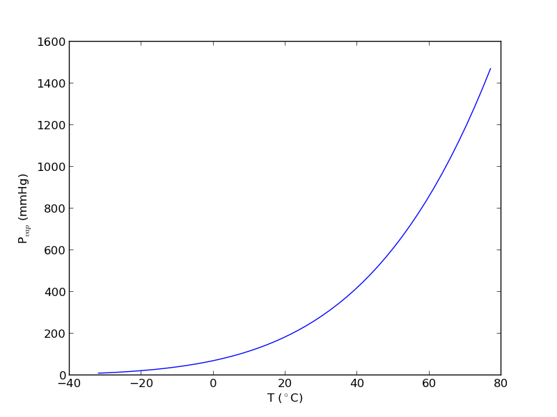
We will use the data to find the temperature at which the vapor pressure of acetone is 400 mmHg.

We use numpy.loadtxt to read the file, and tell the function the format of each column. This creates a special kind of record array which we can access data by field name.

import numpy as np
import matplotlib.pyplot as plt

data = np.loadtxt('data/antoine_data.dat',
                  dtype=[('id', np.int),
                         ('formula', 'S8'),
                         ('name', 'S28'),
                         ('A', np.float),
                         ('B', np.float),
                         ('C', np.float),
                         ('Tmin', np.float),
                         ('Tmax', np.float),
                         ('??', 'S4'),
                         ('?', 'S4')],
                  skiprows=7)

names = data['name']

acetone, = data[names == 'acetone']

# for readability we unpack the array into variables
id, formula, name, A, B, C, Tmin, Tmax, u1, u2 = acetone

T = np.linspace(Tmin, Tmax)
P = 10**(A - B / ( T + C))
plt.plot(T, P)
plt.xlabel('T ($^\circ$C)')
plt.ylabel('P$_{vap}$ (mmHg)')

# Find T at which Pvap = 400 mmHg
# from our graph we might guess T ~ 40 ^{\circ}C

def objective(T):
    return 400 - 10**(A - B / (T + C))

from scipy.optimize import fsolve
Tsol, = fsolve(objective, 40)
print Tsol
print 'The vapor pressure is 400 mmHg at T = {0:1.1f} degC'.format(Tsol)

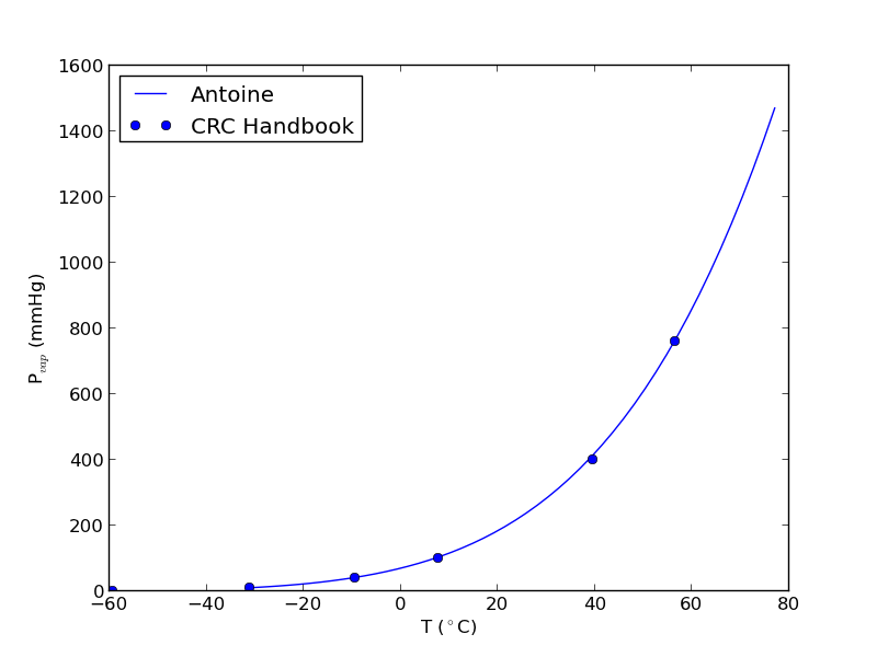
#Plot CRC data http://en.wikipedia.org/wiki/Acetone_%28data_page%29#Vapor_pressure_of_liquid
# We only include the data for the range where the Antoine fit is valid.

Tcrc  = [-59.4,         -31.1,  -9.4,   7.7,    39.5,   56.5]
Pcrc = [        1,      10,     40,     100,    400,    760]

plt.plot(Tcrc, Pcrc, 'bo')
plt.legend(['Antoine','CRC Handbook'], loc='best')
plt.savefig('images/antoine-2.png')
38.6138198197
The vapor pressure is 400 mmHg at T = 38.6 degC

This result is close to the value reported here (39.5 degC), from the CRC Handbook. The difference is probably that the value reported in the CRC is an actual experimental number.

Copyright (C) 2013 by John Kitchin. See the License for information about copying.
org-mode source

Discuss on Twitter

Finding equilibrium conversion

| categories: nonlinear algebra | tags:

A common problem to solve in reaction engineering is finding the equilibrium conversion.1 A typical problem to solve is the following nonlinear equation:

\(1.44 = \frac{X_e^2}{(1-X_e)^2}\)

To solve this we create a function:

\(f(X_e)=0=1.44 - \frac{X_e^2}{(1-X_e)^2}\)

and use a nonlinear solver to find the value of \(X_e\) that makes this function equal to zero. We have to provide an initial guess. Chemical intuition suggests that the solution must be between 0 and 1, and mathematical intuition suggests the solution might be near 0.5 (which would give a ratio near 1).

Here is our solution.

from scipy.optimize import fsolve

def func(Xe):
    z = 1.44 - (Xe**2)/(1-Xe)**2
    return z

X0 = 0.5
Xe, = fsolve(func, X0)
print('The equilibrium conversion is X = {0:1.2f}'.format(Xe))
The equilibrium conversion is X = 0.55

Copyright (C) 2013 by John Kitchin. See the License for information about copying.
org-mode source

Discuss on Twitter

Counting roots

| categories: nonlinear algebra | tags:

Matlab post The goal here is to determine how many roots there are in a nonlinear function we are interested in solving. For this example, we use a cubic polynomial because we know there are three roots.

$$f(x) = x^3 + 6x^2 - 4x -24$$

1 Use roots for this polynomial

This ony works for a polynomial, it does not work for any other nonlinear function.

import numpy as np
print np.roots([1, 6, -4, -24])
[-6.  2. -2.]

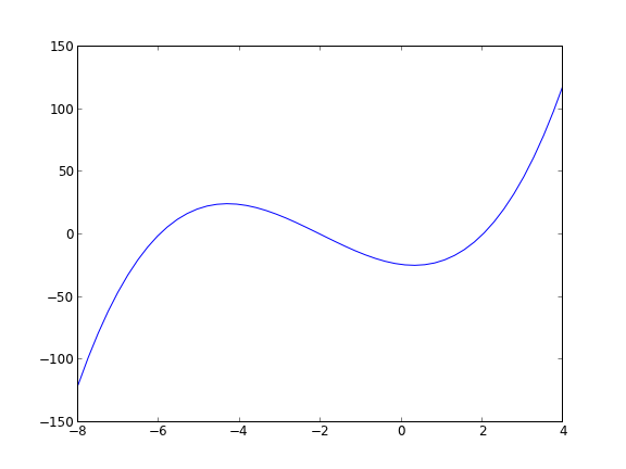
Let us plot the function to see where the roots are.

import numpy as np
import matplotlib.pyplot as plt

x = np.linspace(-8, 4)
y = x**3 + 6 * x**2 - 4*x - 24
plt.plot(x, y)
plt.savefig('images/count-roots-1.png')

Now we consider several approaches to counting the number of roots in this interval. Visually it is pretty easy, you just look for where the function crosses zero. Computationally, it is tricker.

2 method 1

Count the number of times the sign changes in the interval. What we have to do is multiply neighboring elements together, and look for negative values. That indicates a sign change. For example the product of two positive or negative numbers is a positive number. You only get a negative number from the product of a positive and negative number, which means the sign changed.

import numpy as np
import matplotlib.pyplot as plt

x = np.linspace(-8, 4)
y = x**3 + 6 * x**2 - 4*x - 24

print np.sum(y[0:-2] * y[1:-1] < 0)
3

This method gives us the number of roots, but not where the roots are.

3 Method 2

Using events in an ODE solver python can identify events in the solution to an ODE, for example, when a function has a certain value, e.g. f(x) = 0. We can take advantage of this to find the roots and number of roots in this case. We take the derivative of our function, and integrate it from an initial starting point, and define an event function that counts zeros.

$$f'(x) = 3x^2 + 12x - 4$$

with f(-8) = -120

import numpy as np
from pycse import odelay

def fprime(f, x):
    return 3.0 * x**2 + 12.0*x - 4.0

def event(f, x):
    value = f # we want f = 0
    isterminal = False
    direction = 0
    return value, isterminal, direction

xspan = np.linspace(-8, 4)
f0 = -120

X, F, TE, YE, IE = odelay(fprime, f0, xspan, events=[event])
for te, ye in zip(TE, YE):
    print 'root found at x = {0: 1.3f}, f={1: 1.3f}'.format(te, ye)
root found at x = -6.000, f=-0.000
root found at x = -2.000, f=-0.000
root found at x =  2.000, f= 0.000

Copyright (C) 2013 by John Kitchin. See the License for information about copying.

org-mode source

Discuss on Twitter

Basic math

| categories: math, python | tags:

Python is a basic calculator out of the box. Here we consider the most basic mathematical operations: addition, subtraction, multiplication, division and exponenetiation. we use the to get the output. For now we consider integers and float numbers. An integer is a plain number like 0, 10 or -2345. A float number has a decimal in it. The following are all floats: 1.0, -9., and 3.56. Note the trailing zero is not required, although it is good style.

print 2 + 4
print 8.1 - 5
6
3.1

Multiplication is equally straightforward.

print 5 * 4
print 3.1*2
20
6.2

Division is almost as straightforward, but we have to remember that integer division is not the same as float division. Let us consider float division first.

print 4.0 / 2.0
print 1.0/3.1
2.0
0.322580645161

Now, consider the integer versions:

print 4 / 2
print 1/3
2
0

The first result is probably what you expected, but the second may come as a surprise. In integer division the remainder is discarded, and the result is an integer.

Exponentiation is also a basic math operation that python supports directly.

print 3.**2
print 3**2
print 2**0.5
9.0
9
1.41421356237

Other types of mathematical operations require us to import functionality from python libraries. We consider those in the next section.

Copyright (C) 2013 by John Kitchin. See the License for information about copying.

org-mode source

Discuss on Twitter
« Previous Page -- Next Page »