Using autograd for error propagation

| categories: uncertainty, autograd | tags:

Back in 2013 I wrote about using the uncertainties package to propagate uncertainties. The problem setup was for finding the uncertainty in the exit concentration from a CSTR when there are uncertainties in the other parameters. In this problem we were given this information about the parameters and their uncertainties.

Parameter value σ
Fa0 5 0.05
v0 10 0.1
V 66000 100
k 3 0.2

The exit concentration is found by solving this equation:

\(0 = Fa0 - v0 * Ca - k * Ca**2 * V\)

So the question was what is Ca, and what is the uncertainty on it? Finding Ca is easy with fsolve.

from scipy.optimize import fsolve

Fa0 = 5.0
v0 = 10.0

V = 66000.0
k = 3.0

def func(Ca, v0, k, Fa0, V):
    "Mole balance for a CSTR. Solve this equation for func(Ca)=0"
    Fa = v0 * Ca     # exit molar flow of A
    ra = -k * Ca**2  # rate of reaction of A L/mol/h
    return Fa0 - Fa + V * ra

Ca, = fsolve(func, 0.1 * Fa0 / v0, args=(v0, k, Fa0, V))
Ca
0.0050000000000000001

The uncertainty on Ca is a little trickier. A simplified way to estimate it is:

\(\sigma_{Ca} = \sqrt{(dCa/dv0)^2 \sigma_{v0}^2 + (dCa/dv0)^2 \sigma_{v0}^2 + (dCa/dFa0)^2 \sigma_{Fa0}^2 + (dCa/dV)^2 \sigma_{V}^2}\)

We know the σ_i for each input, we just need those partial derivatives. However, we only have the implicit function we used to solve for Ca, and I do not want to do the algebra to solve for Ca. Luckily, we previously worked out how to get these derivatives from an implicit function using autograd. We just need to loop through the arguments, get the relevant derivatives, and accumulate the product of the squared derivatives and errors. Finally, take the square root of that sum.

import autograd.numpy as np
from autograd import grad

# these are the uncertainties on the inputs
s = [None, 0.1, 0.2, 0.05, 100]

S2 = 0.0

dfdCa = grad(func, 0)
for i in range(1, 5):
    dfdarg2 = grad(func, i)
    dCadarg2 = -dfdarg2(Ca, v0, k, Fa0, V) / dfdCa(Ca, v0, k, Fa0, V)
    S2 += dCadarg2**2 * s[i]**2

Ca_s = np.sqrt(S2)
print(f'Ca = {Ca:1.5f} +\- {Ca_s}')
Ca = 0.00500 +\- 0.00016776432898276802


That is the same uncertainty estimate the quantities package provided. One benefit here is I did not have to do the somewhat complicated wrapping procedure around fsolve that was required with uncertainties to get this. On the other hand, I did have to derive the formula and implement them. It worked fine here, since we have an implicit function and a way to get the required derivatives. It could take some work to do this with the exit concentration of a PFR, which requires an integrator. Maybe that differentiable integrator will come in handy again!

Copyright (C) 2018 by John Kitchin. See the License for information about copying.

org-mode source

Org-mode version = 9.1.14

Discuss on Twitter

Visualizing uncertainty in linear regression

| categories: uncertainty, data analysis | tags:

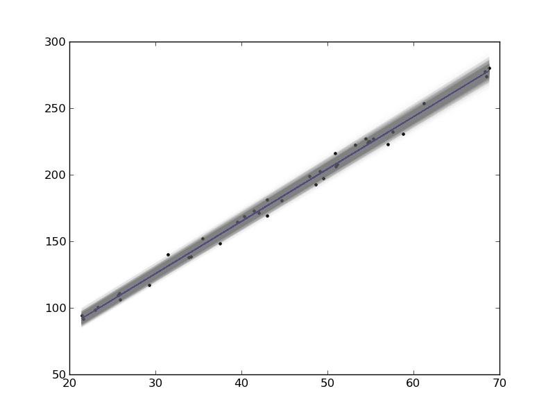
In this example, we show how to visualize uncertainty in a fit. The idea is to fit a model to data, and get the uncertainty in the model parameters. Then we sample the parameters according to the normal distribution, and plot the corresponding distribution of models. We use transparent lines and allow the overlap to indicate the density of the fits.

The data is stored in a text file download PT.txt , with the following structure:

Run          Ambient                            Fitted
 Order  Day  Temperature  Temperature  Pressure    Value    Residual
  1      1      23.820      54.749      225.066   222.920     2.146
...

We need to read the data in, and perform a regression analysis on P vs. T. In python we start counting at 0, so we actually want columns 3 and 4.

import numpy as np
import matplotlib.pyplot as plt
from pycse import regress

data = np.loadtxt('../../pycse/data/PT.txt', skiprows=2)
T = data[:, 3]
P = data[:, 4]

A = np.column_stack([T**0, T])

p, pint, se = regress(A, P, 0.05)

print p, pint, se
plt.plot(T, P, 'k.')
plt.plot(T, np.dot(A, p))

# Now we plot the distribution of possible lines
N = 2000
B = np.random.normal(p[0], se[0], N)
M = np.random.normal(p[1], se[1], N)
x = np.array([min(T), max(T)])

for b,m in zip(B, M):
    plt.plot(x, m*x + b, '-', color='gray', alpha=0.02)
plt.savefig('images/plotting-uncertainty.png')
[ 7.74899739  3.93014044] [[  2.97964903  12.51834576]
 [  3.82740876   4.03287211]] [ 2.35384765  0.05070183]

Here you can see 2000 different lines that have some probability of being correct. The darkest gray is near the fit, as expected; the darker the gray the more probable it is the line. This is a qualitative way of judging the quality of the fit.

Note, this is not the prediction error that we are plotting, that is the uncertainty in where a predicted y-value is.

Copyright (C) 2013 by John Kitchin. See the License for information about copying.

org-mode source

Discuss on Twitter

Uncertainty in the solution of an ODE

| categories: uncertainty, ode | tags:

Our objective in this post is to examine the effects of uncertainty in parameters that define an ODE on the integrated solution of the ODE. My favorite method for numerical uncertainty analysis is Monte Carlo simulation because it is easy to code and usually easy to understand. We take that approach first.

The problem to solve is to estimate the conversion in a constant volume batch reactor with a second order reaction \(A \rightarrow B\), and the rate law: \(-r_A = k C_A^2\), after one hour of reaction. There is 5% uncertainty in the rate constant \(k=0.001\) and in the initial concentration \(C_{A0}=1\).

The relevant differential equation is:

\(\frac{dX}{dt} = -r_A /C_{A0}\).

We have to assume that 5% uncertainty refers to a normal distribution of error that has a standard deviation of 5% of the mean value.

from scipy.integrate import odeint
import numpy as np

N = 1000

K = np.random.normal(0.001, 0.05*0.001, N)
CA0 = np.random.normal(1, 0.05*1, N)

X = [] # to store answer in
for k, Ca0 in zip(K, CA0):
    # define ODE
    def ode(X, t):
        ra = -k * (Ca0 * (1 - X))**2
        return -ra / Ca0
    
    X0 = 0
    tspan = np.linspace(0,3600)

    sol = odeint(ode, X0, tspan)

    X += [sol[-1][0]]

s = 'Final conversion at one hour is {0:1.3f} +- {1:1.3f} (1 sigma)'
print s.format(np.average(X),
               np.std(X))
Final conversion at one hour is 0.782 +- 0.013 (1 sigma)

See, it is not too difficulty to write. It is however, a little on the expensive side to run, since we typically need 1e3-1e6 samples to get the statistics reasonable. Let us try the uncertainties package too. For this we have to wrap a function that takes uncertainties and returns a single float number.

from scipy.integrate import odeint
import numpy as np
import uncertainties as u

k = u.ufloat(0.001, 0.05*0.001)
Ca0 = u.ufloat(1.0, 0.05)

@u.wrap
def func(k, Ca0):
    # define the ODE
    def ode(X, t):
        ra = -k * (Ca0 * (1 - X))**2
        return -ra / Ca0
    
    X0 = 0 # initial condition
    tspan = np.linspace(0, 3600)
    # integrate it
    sol = odeint(ode, X0, tspan)
    return sol[-1][0]

result = func(k, Ca0)
s = 'Final conversion at one hour is {0}(1 sigma)'
print s.format(result)
Final conversion at one hour is 0.783+/-0.012(1 sigma)

This is about the same amount of code as the Monte Carlo approach, but it runs much faster, and gets approximately the same results. You have to remember the wrapping technique, since the uncertainties package does not run natively with the odeint function.

Copyright (C) 2013 by John Kitchin. See the License for information about copying.

org-mode source

Discuss on Twitter

Uncertainty in an integral equation

| categories: math, uncertainty | tags:

In a previous example, we solved for the time to reach a specific conversion in a batch reactor. However, it is likely there is uncertainty in the rate constant, and possibly in the initial concentration. Here we examine the effects of that uncertainty on the time to reach the desired conversion.

To do this we have to write a function that takes arguments with uncertainty, and wrap the function with the uncertainties.wrap decorator. The function must return a single float number (current limitation of the uncertainties package). Then, we simply call the function, and the uncertainties from the inputs will be automatically propagated to the outputs. Let us say there is about 10% uncertainty in the rate constant, and 1% uncertainty in the initial concentration.

from scipy.integrate import quad
import uncertainties as u

k = u.ufloat((1.0e-3, 1.0e-4))
Ca0 = u.ufloat((1.0, 0.01))# mol/L

@u.wrap
def func(k, Ca0):
    def integrand(X):
        return 1./(k*Ca0)*(1./(1-X)**2)
    integral, abserr = quad(integrand, 0, 0.9)
    return integral

sol = func(k, Ca0)
print 't = {0} seconds ({1} hours)'.format(sol, sol/3600)
t = 9000.0+/-904.488801332 seconds (2.5+/-0.251246889259 hours)

The result shows about a 10% uncertainty in the time, which is similar to the largest uncertainty in the inputs. This information should certainly be used in making decisions about how long to actually run the reactor to be sure of reaching the goal. For example, in this case, running the reactor for 3 hours (that is roughly + 2σ) would ensure at a high level of confidence (approximately 95% confidence) that you reach at least 90% conversion.

Copyright (C) 2013 by John Kitchin. See the License for information about copying.

org-mode source

Discuss on Twitter

Uncertainty in polynomial roots - Part II

| categories: uncertainty, data analysis | tags:

We previously looked at uncertainty in polynomial roots where we had an analytical formula for the roots of the polynomial, and we knew the uncertainties in the polynomial parameters. It would be inconvenient to try this for a cubic polynomial, although there may be formulas for the roots. I do not know of there are general formulas for the roots of a 4th order polynomial or higher.

Unfortunately, we cannot use the uncertainties package out of the box directly here.

import uncertainties as u
import numpy as np
c, b, a = [-0.99526746, -0.011546,    1.00188999]
sc, sb, sa = [ 0.0249142,   0.00860025,  0.00510128]

A = u.ufloat((a, sa))
B = u.ufloat((b, sb))
C = u.ufloat((c, sc))

print np.roots([A, B, C])
>>> >>> >>> >>> >>> >>> >>> >>> Traceback (most recent call last):
  File "<stdin>", line 1, in <module>
  File "c:\Users\jkitchin\AppData\Local\Enthought\Canopy\User\lib\site-packages\numpy\lib\polynomial.py", line 218, in roots
    p = p.astype(float)
  File "c:\Users\jkitchin\AppData\Local\Enthought\Canopy\User\lib\site-packages\uncertainties\__init__.py", line 1257, in raise_error
    % (self.__class__, coercion_type))
TypeError: can't convert an affine function (<class 'uncertainties.Variable'>) to float; use x.nominal_value

To make some progress, we have to understand how the numpy.roots function works. It constructs a Companion matrix, and the eigenvalues of that matrix are the same as the roots of the polynomial.

import numpy as np

c0, c1, c2 = [-0.99526746, -0.011546,    1.00188999]

p = np.array([c2, c1, c0])
N = len(p)

# we construct the companion matrix like this
# see https://github.com/numpy/numpy/blob/v1.7.0/numpy/lib/polynomial.py#L220
# for this code.
# build companion matrix and find its eigenvalues (the roots)
A = np.diag(np.ones((N-2,), p.dtype), -1)
A[0, :] = -p[1:] / p[0]

print A

roots = np.linalg.eigvals(A)
print roots
[[ 0.01152422  0.99338996]
 [ 1.          0.        ]]
[ 1.00246827 -0.99094405]

This definition of the companion matrix is a little different than the one here, but primarily in the scaling of the coefficients. That does not seem to change the eigenvalues, or the roots.

Now, we have a path to estimate the uncertainty in the roots. Since we know the polynomial coefficients and their uncertainties from the fit, we can use Monte Carlo sampling to estimate the uncertainty in the roots.

import numpy as np
import uncertainties as u

c, b, a = [-0.99526746, -0.011546,    1.00188999]
sc, sb, sa = [ 0.0249142,   0.00860025,  0.00510128]

NSAMPLES = 100000
A = np.random.normal(a, sa, (NSAMPLES, ))
B = np.random.normal(b, sb, (NSAMPLES, ))
C = np.random.normal(c, sc, (NSAMPLES, ))

roots = [[] for i in range(NSAMPLES)]

for i in range(NSAMPLES):
    p = np.array([A[i], B[i], C[i]])
    N = len(p)
    
    M = np.diag(np.ones((N-2,), p.dtype), -1)
    M[0, :] = -p[1:] / p[0]
    r = np.linalg.eigvals(M)
    r.sort()  # there is no telling what order the values come out in
    roots[i] = r
    
avg = np.average(roots, axis=0)
std = np.std(roots, axis=0)

for r, s in zip(avg, std):
    print '{0: f} +/- {1: f}'.format(r, s)
-0.990949 +/-  0.013435
 1.002443 +/-  0.013462

Compared to our previous approach with the uncertainties package where we got:

: -0.990944048037+/-0.0134208013339
:  1.00246826738 +/-0.0134477390832

the agreement is quite good! The advantage of this approach is that we do not have to know the formula for the roots of higher order polynomials to estimate the uncertainty in the roots. The downside is we have to evaluate the eigenvalues of a matrix a large number of times to get good estimates of the uncertainty. For high power polynomials this could be problematic. I do not currently see a way around this, unless it becomes possible to get the uncertainties package to propagate through the numpy.eigvals function. It is possible to wrap some functions with uncertainties, but so far only functions that return a single number.

There are some other potential problems with this approach. It is assumed that the accuracy of the eigenvalue solver is much better than the uncertainty in the polynomial parameters. You have to use some judgment in using these uncertainties. We are approximating the uncertainties of a nonlinear problem. In other words, the uncertainties of the roots are not linearly dependent on the uncertainties of the polynomial coefficients.

It is possible to wrap some functions with uncertainties, but so far only functions that return a single number. Here is an example of getting the nth root and its uncertainty.

import uncertainties as u
import numpy as np

@u.wrap
def f(n=0, *P):
    ''' compute the nth root of the polynomial P and the uncertainty of the root'''
    p =  np.array(P)
    N = len(p)
    
    M = np.diag(np.ones((N-2,), p.dtype), -1)
    M[0, :] = -p[1:] / p[0]
    r = np.linalg.eigvals(M)
    r.sort()  # there is no telling what order the values come out in
    return r[n]

# our polynomial coefficients and standard errors
c, b, a = [-0.99526746, -0.011546,    1.00188999]
sc, sb, sa = [ 0.0249142,   0.00860025,  0.00510128]

A = u.ufloat((a, sa))
B = u.ufloat((b, sb))
C = u.ufloat((c, sc))

for result in [f(n, A, B, C) for n in [0, 1]]:
    print result
-0.990944048037+/-0.013420800377
1.00246826738+/-0.0134477388218

It is good to see this is the same result we got earlier, with a lot less work (although we do have to solve it for each root, which is a bit redundant)! It is a bit more abstract though, and requires a specific formulation of the function for the wrapper to work.

Copyright (C) 2013 by John Kitchin. See the License for information about copying.

org-mode source

Discuss on Twitter
Next Page ยป