Using autograd in nonlinear regression
Posted November 17, 2017 at 07:49 AM | categories: regression, autograd, python | tags:
Table raw-data contains the energy as a function of volume for some solid material from a set of density functional theory calculations. Our goal is to fit the Murnaghan equation of state to this data. The model is moderately nonlinear. I have previously done this with the standard nonlinear regression functions in scipy, so today we will use autograd along with a builtin optimizer to minimize an objective function to achieve the same thing.
The basic idea is we define an objective function, in this case the summed squared errors between predicted values from the model and known values from our data. The objective function takes two arguments: the model parameters, and the "step". This function signature is a consequence of the built in optimizer we use; it expects that signature (it is useful for batch training, but we will not use that here). We use autograd to create a gradient of the objective function which the adam optimizer will use to vary the parameters with the goal of minimizing the objective function.
The adam optimizer function takes as one argument a callback function, which we call summary to print out intermediate results during the convergence. We run the optimizer in a loop because the optimizer runs a fixed number of steps on each call. We check if the objective function is sufficiently small, and if it is we break out.
import autograd.numpy as np
from autograd import grad
from autograd.misc.optimizers import adam

np.set_printoptions(precision=3, suppress=True)

# input data
Vinput = np.array([row[0] for row in data])
Eknown = np.array([row[1] for row in data])

def Murnaghan(pars, vol):
    '''
    given a vector of parameters and volumes, return a vector of energies.
    equation From PRB 28,5480 (1983)
    '''
    E0, B0, BP, V0 = pars
    E = E0 + B0 * vol / BP * (((V0 / vol)**BP) / (BP - 1.0) + 1.0) - V0 * B0 / (BP - 1.)
    return E

def objective(pars, step):
    "This is what we want to minimize by varying the pars."
    predicted = Murnaghan(pars, Vinput)
    # Note Eknown is not defined in this function scope
    errors = Eknown - predicted
    return np.sum(errors**2)

objective_grad = grad(objective)

def summary(pars, step, gradient):
    # Note i, N are not defined in this function scope
    if step % N == 0:
        print('step {0:5d}: {1:1.3e}'.format(i * N + step,
                                             objective(pars, step)))

pars = np.array([-400, 0.5, 2, 210]) # The initial guess
N = 200 # num of steps to take on each optimization
learning_rate = 0.001
for i in range(100):
    pars = adam(objective_grad, pars, step_size=learning_rate,
                num_iters=N, callback=summary)
    SSE = objective(pars, None)
    if SSE < 0.00002:
        print('Tolerance met.', SSE)
        break
print(pars)
step     0: 3.127e+02
step   200: 1.138e+02
step   400: 2.011e+01
step   600: 1.384e+00
step   800: 1.753e-01
step  1000: 2.044e-03
step  1200: 1.640e-03
step  1400: 1.311e-03
step  1600: 1.024e-03
step  1800: 7.765e-04
step  2000: 5.698e-04
step  2200: 4.025e-04
step  2400: 2.724e-04
step  2600: 1.762e-04
step  2800: 1.095e-04
step  3000: 6.656e-05
step  3200: 3.871e-05
step  3400: 2.359e-05
('Tolerance met.', 1.5768901008364176e-05)
[-400.029    0.004    4.032  211.847]
There are some subtleties in the code above. One is the variables that are used kind of all over the place, which is noted in a few places. Those could get tricky to keep track of. Another is the variable I called learning_rate. I borrowed that terminology from the machine learning community. It is the step_size in this implementation of the optimizer. If you make it too large, the objective function doesn't converge, but if you set it too small, it will take a long time to converge. Note that it took at about 3400 steps of "training". This is a lot more than is typically required by something like pycse.nlinfit. This isn't the typical application for this approach to regression. More on that another day.
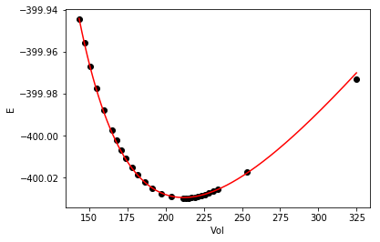
As with any fit, it is wise to check it out at least graphically. Here is the fit and data.
%matplotlib inline
import matplotlib
matplotlib.rc('axes.formatter', useoffset=False)
import matplotlib.pyplot as plt

plt.plot(Vinput, Eknown, 'ko', label='known')

vinterp = np.linspace(Vinput.min(), Vinput.max(), 200)

plt.plot(vinterp, Murnaghan(pars, vinterp), 'r-', label='predicted')
plt.xlabel('Vol')
plt.ylabel('E')

The fit looks pretty good.
| volume | energy |
|---|---|
| 324.85990899 | -399.9731688470 |
| 253.43999457 | -400.0172393178 |
| 234.03826687 | -400.0256270548 |
| 231.12159387 | -400.0265690700 |
| 228.40609504 | -400.0273551120 |
| 225.86490337 | -400.0280030862 |
| 223.47556626 | -400.0285313450 |
| 221.21992353 | -400.0289534593 |
| 219.08319566 | -400.0292800709 |
| 217.05369547 | -400.0295224970 |
| 215.12089909 | -400.0296863867 |
| 213.27525144 | -400.0297809256 |
| 211.51060823 | -400.0298110000 |
| 203.66743321 | -400.0291665573 |
| 197.07888649 | -400.0275017142 |
| 191.39717952 | -400.0250998136 |
| 186.40163591 | -400.0221371852 |
| 181.94435510 | -400.0187369863 |
| 177.92077043 | -400.0149820198 |
| 174.25380090 | -400.0109367042 |
| 170.88582166 | -400.0066495100 |
| 167.76711189 | -400.0021478258 |
| 164.87096104 | -399.9974753449 |
| 159.62553397 | -399.9876885136 |
| 154.97005460 | -399.9774175487 |
| 150.78475335 | -399.9667603369 |
| 146.97722201 | -399.9557686286 |
| 143.49380641 | -399.9445262604 |
Copyright (C) 2017 by John Kitchin. See the License for information about copying.
Org-mode version = 9.1.2