Posting articles to CiteULike from bibtex

| categories: citeulike, python, emacs | tags:

Table of Contents

I have been using CiteULike for a while now to keep a list of articles that are probably worth reading. Basically, each month I get a table of contents from many journals, and as I read through them, if an article catches my attention I add it to my CiteULike account.

This list is not synchronized with my bibtex database however. These serve different purposes. The CiteULike list is for articles that are probably worth reading, while the bibtex file contains articles I am probably going to cite. It should be that every article in my bibtex file is on CiteULike, but not necessarily the other way around. The problem is I do not have a way to push files from my bibtex file to CiteULike easily.

CiteULike allows you to import a bibtex file though. I want to explore automatically importing a bibtex file by simulating the form. We need a set of cookies to make this happen so CiteULike knows who we are. I stored my username and password in a file called citeulike.json and use them to get cookies that I save here in a pickle file. I think this cookie gives you access to your CiteULike account, so it should be kept secret.

import json, pickle, requests

with open('citeulike.json') as f:
    d = json.loads(f.read())

url = 'http://www.citeulike.org/login.do'

data = "username={0}&password={1}&perm=1".format(d['username'], d['password'])

r = requests.post(url, data=data, allow_redirects=False)

with open('cookies.pckl', 'wb') as f:
    pickle.dump(r.cookies, f)

By inspecting the import page with Firebug, I constructed this http request to upload a bibtex string.

import pickle, requests

# reload cookies
with open('cookies.pckl', 'rb') as f:
    cookies = pickle.load(f)

url = 'http://www.citeulike.org/profile/jkitchin/import_do'

bibtex = '''
@article{zhuo-2010-co2-induc,
  author =       {Zhuo, Shengchi and Huang, Yongmin and Peng, Changjun
                  and Liu, Honglai and Hu, Ying and Jiang, Jianwen},
  title =        {CO2-Induced Microstructure Transition of Surfactant
                  in Aqueous Solution: Insight from Molecular Dynamics
                  Simulation},
  journal =      {The Journal of Physical Chemistry B},
  volume =       114,
  number =       19,
  pages =        {6344-6349},
  year =         2010,
  doi =          {10.1021/jp910253b},
  URL =          {http://pubs.acs.org/doi/abs/10.1021/jp910253b},
  eprint =       {http://pubs.acs.org/doi/pdf/10.1021/jp910253b}
}'''

data = {'pasted':bibtex,
        'to_read':2,
        'tag_parsing':'simple',
        'strip_brackets':'no',
        'update_id':'bib-key',
        'btn_bibtex':'Import BibTeX file ...'}

headers = {'content-type': 'multipart/form-data',
           'User-Agent':'jkitchin/johnrkitchin@gmail.com bibtexupload'}

r = requests.post(url, headers=headers, data=data, cookies=cookies, files={})

The result is that article is now listed in my CiteULike at http://www.citeulike.org/user/jkitchin/article/12728895 . This opens the possibility of integrating this into my bibtex workflow. I could implement this in emacs-lisp, and have it automatically upload new entries in the bibtex file to CiteULike.

1 Doing this in emacs

I think the easiest thing to do here is to write a python script that takes the bibtex string and posts it. We will use emacs to get the bibtex string. We will use the example at http://ergoemacs.org/emacs/elisp_perl_wrapper.html to put this together. This example uses an external script that takes a string on stdin, and returns a result on stdout.

We will run the function in a bibtex buffer. We will narrow the buffer to the current entry, and use that to define the boundaries of the string. We do the command in a temp-buffer to prevent it from modifying our bibtex file. There is some way to make the command not do this with optional arguments, but I did not figure it out. It is a little ugly I had to use an absolute path below. An alternative would be to put the script into a directory on your path. Here is the function.

(defun j/upload-bibtex-entry-to-citeulike ()
  "get bibtex string and submit to citeulike"
  (interactive)
  (save-restriction
    (bibtex-narrow-to-entry)
    (let ((startpos (point-min))
          (endpos (point-max))
          (bibtex-string (buffer-string))
          (script "python c:/Users/jkitchin/Dropbox/blogofile-jkitchin.github.com/_blog/upload_bibtex_citeulike.py"))
      (with-temp-buffer (insert bibtex-string)
                        (shell-command-on-region (point-min) (point-max) script t nil nil t)))))

Now, let us define the python script.

#!python
import pickle, requests, sys

# reload cookies
with open('c:/Users/jkitchin/Dropbox/blogofile-jkitchin.github.com/_blog/cookies.pckl', 'rb') as f:
    cookies = pickle.load(f)

url = 'http://www.citeulike.org/profile/jkitchin/import_do'

bibtex = sys.stdin.read()

data = {'pasted':bibtex,
        'to_read':2,
        'tag_parsing':'simple',
        'strip_brackets':'no',
        'update_id':'bib-key',
        'btn_bibtex':'Import BibTeX file ...'}

headers = {'content-type': 'multipart/form-data',
           'User-Agent':'jkitchin/johnrkitchin@gmail.com bibtexupload'}

r = requests.post(url, headers=headers, data=data, cookies=cookies, files={})

That is it. Now, in my bibtex file with the cursor in an entry, I type M-x j/upload-bibtex-entry-to-citeulike, and a few seconds later the entry has been uploaded!

Copyright (C) 2013 by John Kitchin. See the License for information about copying.
org-mode source

Discuss on Twitter

Interesting online python sites

| categories: python | tags:

I have come across some very interesting online, interactive python sites recently.

Here are a few others I came across:

Copyright (C) 2013 by John Kitchin. See the License for information about copying.
org-mode source

Discuss on Twitter

Advanced function creation

| categories: python | tags:

Python has some nice features in creating functions. You can create default values for variables, have optional variables and optional keyword variables. In this function f(a,b), a and b are called positional arguments, and they are required, and must be provided in the same order as the function defines.

If we provide a default value for an argument, then the argument is called a keyword argument, and it becomes optional. You can combine positional arguments and keyword arguments, but positional arguments must come first. Here is an example.

def func(a, n=2):
    "compute the nth power of a"
    return a**n

# three different ways to call the function
print func(2)
print func(2, 3)
print func(2, n=4)
4
8
16

In the first call to the function, we only define the argument a, which is a mandatory, positional argument. In the second call, we define a and n, in the order they are defined in the function. Finally, in the third call, we define a as a positional argument, and n as a keyword argument.

If all of the arguments are optional, we can even call the function with no arguments. If you give arguments as positional arguments, they are used in the order defined in the function. If you use keyword arguments, the order is arbitrary.

def func(a=1, n=2):
    "compute the nth power of a"
    return a**n

# three different ways to call the function
print func()
print func(2, 4)
print func(n=4, a=2)
1
16
16

It is occasionally useful to allow an arbitrary number of arguments in a function. Suppose we want a function that can take an arbitrary number of positional arguments and return the sum of all the arguments. We use the syntax *args to indicate arbitrary positional arguments. Inside the function the variable args is a tuple containing all of the arguments passed to the function.

def func(*args):
    sum = 0
    for arg in args:
        sum += arg
    return sum

print func(1, 2, 3, 4)
10

A more “functional programming” version of the last function is given here. This is an advanced approach that is less readable to new users, but more compact and likely more efficient for large numbers of arguments.

import operator
def func(*args):
    return reduce(operator.add, args)
print func(1, 2, 3, 4)
10

It is possible to have arbitrary keyword arguments. This is a common pattern when you call another function within your function that takes keyword arguments. We use **kwargs to indicate that arbitrary keyword arguments can be given to the function. Inside the function, kwargs is variable containing a dictionary of the keywords and values passed in.

def func(**kwargs):
    for kw in kwargs:
        print '{0} = {1}'.format(kw, kwargs[kw])

func(t1=6, color='blue')
color = blue
t1 = 6

A typical example might be:

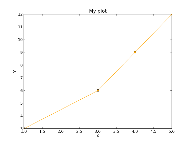
import matplotlib.pyplot as plt

def myplot(x, y, fname=None, **kwargs):
    "make plot of x,y. save to fname if not None. provide kwargs to plot"
    plt.plot(x, y, **kwargs)
    plt.xlabel('X')
    plt.ylabel('Y')
    plt.title('My plot')
    if fname:
        plt.savefig(fname)
    else:
        plt.show()

x = [1, 3, 4, 5]
y = [3, 6, 9, 12]

myplot(x, y, 'images/myfig.png', color='orange', marker='s')

# you can use a dictionary as kwargs
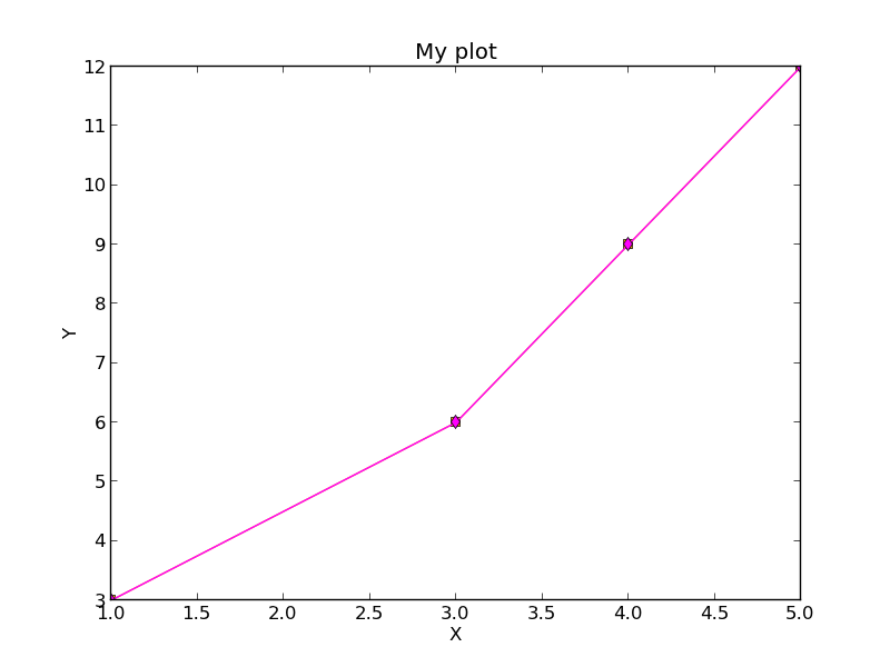
d = {'color':'magenta',
     'marker':'d'}

myplot(x, y, 'images/myfig2.png', **d)

In that example we wrap the matplotlib plotting commands in a function, which we can call the way we want to, with arbitrary optional arguments. In this example, you cannot pass keyword arguments that are illegal to the plot command or you will get an error.

It is possible to combine all the options at once. I admit it is hard to imagine where this would be really useful, but it can be done!

import numpy as np

def func(a, b=2, *args, **kwargs):
    "return a**b + sum(args) and print kwargs"
    for kw in kwargs:
        print 'kw: {0} = {1}'.format(kw, kwargs[kw])

    return a**b + np.sum(args)

print func(2, 3, 4, 5, mysillykw='hahah')
kw: mysillykw = hahah
17

Copyright (C) 2013 by John Kitchin. See the License for information about copying.
org-mode source

Discuss on Twitter

Functions on arrays of values

| categories: python | tags:

It is common to evaluate a function for a range of values. Let us consider the value of the function \(f(x) = \cos(x)\) over the range of \(0 < x < \pi\). We cannot consider every value in that range, but we can consider say 10 points in the range. The nil conveniently creates an array of values.

import numpy as np
print np.linspace(0, np.pi, 10)
[ 0.          0.34906585  0.6981317   1.04719755  1.3962634   1.74532925
  2.0943951   2.44346095  2.7925268   3.14159265]

The main point of using the nil functions is that they work element-wise on elements of an array. In this example, we compute the \(\cos(x)\) for each element of \(x\).

import numpy as np
x = np.linspace(0, np.pi, 10)
print np.cos(x)
[ 1.          0.93969262  0.76604444  0.5         0.17364818 -0.17364818
 -0.5        -0.76604444 -0.93969262 -1.        ]

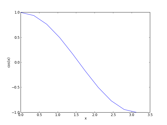
You can already see from this output that there is a root to the equation \(\cos(x) = 0\), because there is a change in sign in the output. This is not a very convenient way to view the results; a graph would be better. We use nil to make figures. Here is an example.

import matplotlib.pyplot as plt
import numpy as np

x = np.linspace(0, np.pi, 10)
plt.plot(x, np.cos(x))
plt.xlabel('x')
plt.ylabel('cos(x)')
plt.savefig('images/plot-cos.png')

This figure illustrates graphically what the numbers above show. The function crosses zero at approximately \(x = 1.5\). To get a more precise value, we must actually solve the function numerically. We use the function nil to do that. More precisely, we want to solve the equation \(f(x) = \cos(x) = 0\). We create a function that defines that equation, and then use nil to solve it.

from scipy.optimize import fsolve 
import numpy as np

def f(x):
    return np.cos(x)

sol, = fsolve(f, x0=1.5) # the comma after sol makes it return a float
print sol
print np.pi / 2
1.57079632679
1.57079632679

We know the solution is π/2.

Copyright (C) 2013 by John Kitchin. See the License for information about copying.
org-mode source

Discuss on Twitter

Defining functions in python

| categories: python | tags:

Compare what's here to the Matlab implementation.

We often need to make functions in our codes to do things.

def f(x):
    "return the inverse square of x"
    return 1.0 / x**2

print f(3)
print f([4,5])
... ... >>> 0.111111111111
Traceback (most recent call last):
  File "<stdin>", line 1, in <module>
  File "<stdin>", line 3, in f
TypeError: unsupported operand type(s) for ** or pow(): 'list' and 'int'

Note that functions are not automatically vectorized. That is why we see the error above. There are a few ways to achieve that. One is to “cast” the input variables to objects that support vectorized operations, such as numpy.array objects.

import numpy as np

def f(x):
    "return the inverse square of x"
    x = np.array(x)
    return 1.0 / x**2

print f(3)
print f([4,5])
>>> ... ... ... ... >>> 0.111111111111
[ 0.0625  0.04  ]

It is possible to have more than one variable.

import numpy as np

def func(x, y):
    "return product of x and y"
    return x * y

print func(2, 3)
print func(np.array([2, 3]), np.array([3, 4]))
6
[ 6 12]

You can define “lambda” functions, which are also known as inline or anonymous functions. The syntax is lambda var:f(var). I think these are hard to read and discourage their use. Here is a typical usage where you have to define a simple function that is passed to another function, e.g. scipy.integrate.quad to perform an integral.

from scipy.integrate import quad
print quad(lambda x:x**3, 0 ,2)
(4.0, 4.440892098500626e-14)

It is possible to nest functions inside of functions like this.

def wrapper(x):
    a = 4
    def func(x, a):
        return a * x

    return func(x, a)

print wrapper(4)
16

An alternative approach is to “wrap” a function, say to fix a parameter. You might do this so you can integrate the wrapped function, which depends on only a single variable, whereas the original function depends on two variables.

def func(x, a):
        return a * x
 
def wrapper(x):
    a = 4
    return func(x, a)

print wrapper(4)
16

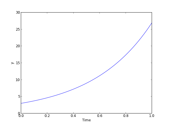
Last example, defining a function for an ode

from scipy.integrate import odeint
import numpy as np
import matplotlib.pyplot as plt

k = 2.2
def myode(t,y):
    "ode defining exponential growth"
    return k * t

y0 = 3
tspan = np.linspace(0,1)
y =  odeint(myode, y0, tspan)

plt.plot(tspan, y)
plt.xlabel('Time')
plt.ylabel('y')
plt.savefig('images/funcs-ode.png')

Copyright (C) 2013 by John Kitchin. See the License for information about copying.

org-mode source

Discuss on Twitter
« Previous Page -- Next Page »