The Kitchin Research Group: linear algebra

Rules for transposition

Posted February 27, 2013 at 01:12 PM | categories: linear algebra | tags:

Here are the four rules for matrix multiplication and transposition

$(\mathbf{A}^T)^T = \mathbf{A}$
$(\mathbf{A}+\mathbf{B})^T = \mathbf{A}^T+\mathbf{B}^T$
$(\mathit{c}\mathbf{A})^T = \mathit{c}\mathbf{A}^T$
$(\mathbf{AB})^T = \mathbf{B}^T\mathbf{A}^T$

reference: Chapter 7.2 in Advanced Engineering Mathematics, 9th edition. by E. Kreyszig.

1 The transpose in Python

There are two ways to get the transpose of a matrix: with a notation, and with a function.

import numpy as np
A = np.array([[5, -8, 1],
              [4, 0, 0]])

# function
print np.transpose(A)


# notation
print A.T

[[ 5  4]
 [-8  0]
 [ 1  0]]
[[ 5  4]
 [-8  0]
 [ 1  0]]

2 Rule 1

import numpy as np

A = np.array([[5, -8, 1],
              [4, 0, 0]])

print np.all(A == (A.T).T)

True

3 Rule 2

import numpy as np
A = np.array([[5, -8, 1],
              [4, 0, 0]])

B = np.array([[3, 4, 5], [1, 2,3]])

print np.all( A.T + B.T == (A + B).T)

True

4 Rule 3

import numpy as np
A = np.array([[5, -8, 1],
              [4, 0, 0]])

c = 2.1

print np.all( (c*A).T == c*A.T)

True

5 Rule 4

import numpy as np
A = np.array([[5, -8, 1],
              [4, 0, 0]])

B = np.array([[0, 2],
              [1, 2],
              [6, 7]])

print np.all(np.dot(A, B).T == np.dot(B.T, A.T))

True

6 Summary

That wraps up showing numerically the transpose rules work for these examples.

org-mode source

Discuss on Twitter

Conservation of mass in chemical reactions

Posted February 27, 2013 at 10:54 AM | categories: linear algebra | tags: reaction engineering

Updated March 06, 2013 at 04:27 PM

Matlab post

Atoms cannot be destroyed in non-nuclear chemical reactions, hence it follows that the same number of atoms entering a reactor must also leave the reactor. The atoms may leave the reactor in a different molecular configuration due to the reaction, but the total mass leaving the reactor must be the same. Here we look at a few ways to show this.

We consider the water gas shift reaction : $CO + H_2O \rightleftharpoons H_2 + CO_2$. We can illustrate the conservation of mass with the following equation: $\bf{\nu}\bf{M}=\bf{0}$. Where $\bf{\nu}$ is the stoichiometric coefficient vector and $\bf{M}$ is a column vector of molecular weights. For simplicity, we use pure isotope molecular weights, and not the isotope-weighted molecular weights. This equation simply examines the mass on the right side of the equation and the mass on left side of the equation.

import numpy as np
nu = [-1, -1, 1, 1];
M = [28, 18, 2, 44];
print np.dot(nu, M)

You can see that sum of the stoichiometric coefficients times molecular weights is zero. In other words a CO and H_2O have the same mass as H_2 and CO_2.

For any balanced chemical equation, there are the same number of each kind of atom on each side of the equation. Since the mass of each atom is unchanged with reaction, that means the mass of all the species that are reactants must equal the mass of all the species that are products! Here we look at the number of C, O, and H on each side of the reaction. Now if we add the mass of atoms in the reactants and products, it should sum to zero (since we used the negative sign for stoichiometric coefficients of reactants).

import numpy as np
            # C   O   H
reactants = [-1, -2, -2]
products  = [ 1,  2,  2]

atomic_masses = [12.011, 15.999, 1.0079]  # atomic masses

print np.dot(reactants, atomic_masses) + np.dot(products, atomic_masses)

>>> ... >>> >>> >>> >>> >>> 0.0

That is all there is to mass conservation with reactions. Nothing changes if there are lots of reactions, as long as each reaction is properly balanced, and none of them are nuclear reactions!

org-mode source

Discuss on Twitter

Sums products and linear algebra notation - avoiding loops where possible

Posted February 26, 2013 at 09:00 AM | categories: linear algebra | tags:

Updated February 27, 2013 at 01:12 PM

Matlab comparison

Today we examine some methods of linear algebra that allow us to avoid writing explicit loops in Matlab for some kinds of mathematical operations.

Consider the operation on two vectors $\bf{a}$ and $\bf{b}$.

$$y=\sum\limits_{i=1}^n a_ib_i$$

a = [1 2 3 4 5]

b = [3 6 8 9 10]

1 Old-fashioned way with a loop

We can compute this with a loop, where you initialize y, and then add the product of the ith elements of a and b to y in each iteration of the loop. This is known to be slow for large vectors

a = [1, 2, 3, 4, 5]
b = [3, 6, 8, 9, 10]

sum = 0
for i in range(len(a)):
    sum = sum + a[i] * b[i]
print sum

This is an old fashioned style of coding. A more modern, pythonic approach is:

a = [1, 2, 3, 4, 5]
b = [3, 6, 8, 9, 10]

sum = 0
for x,y in zip(a,b):
    sum += x * y
print sum

2 The numpy approach

The most compact method is to use the methods in numpy.

import numpy as np

a = np.array([1, 2, 3, 4, 5])
b = np.array([3, 6, 8, 9, 10])

print np.sum(a * b)

3 Matrix algebra approach.

The operation defined above is actually a dot product. We an directly compute the dot product in numpy. Note that with 1d arrays, python knows what to do and does not require any transpose operations.

import numpy as np

a = np.array([1, 2, 3, 4, 5])
b = np.array([3, 6, 8, 9, 10])

print np.dot(a, b)

4 Another example

Consider $y = \sum\limits_{i=1}^n w_i x_i^2$. This operation is like a weighted sum of squares. The old-fashioned way to do this is with a loop.

w = [0.1, 0.25, 0.12, 0.45, 0.98];
x = [9, 7, 11, 12, 8];
y = 0
for wi, xi in zip(w,x):
   y += wi * xi**2
print y

162.39

Compare this to the more modern numpy approach.

import numpy as np
w = np.array([0.1, 0.25, 0.12, 0.45, 0.98])
x = np.array([9, 7, 11, 12, 8])
y = np.sum(w * x**2)
print y

162.39

We can also express this in matrix algebra form. The operation is equivalent to $y = \vec{x} \cdot D_w \cdot \vec{x}^T$ where $D_w$ is a diagonal matrix with the weights on the diagonal.

import numpy as np
w = np.array([0.1, 0.25, 0.12, 0.45, 0.98])
x = np.array([9, 7, 11, 12, 8])
y = np.dot(x, np.dot(np.diag(w), x))
print y

162.39

This last form avoids explicit loops and sums, and relies on fast linear algebra routines.

5 Last example

Consider the sum of the product of three vectors. Let $y = \sum\limits_{i=1}^n w_i x_i y_i$. This is like a weighted sum of products.

import numpy as np

w = np.array([0.1, 0.25, 0.12, 0.45, 0.98])
x = np.array([9, 7, 11, 12, 8])
y = np.array([2, 5, 3, 8, 0])

print np.sum(w * x * y)
print np.dot(w, np.dot(np.diag(x), y))

57.71
57.71

6 Summary

We showed examples of the following equalities between traditional sum notations and linear algebra

$$\bf{a}\bf{b}=\sum\limits_{i=1}^n a_ib_i$$

$$\bf{x}\bf{D_w}\bf{x^T}=\sum\limits_{i=1}^n w_ix_i^2$$

$$\bf{x}\bf{D_w}\bf{y^T}=\sum\limits_{i=1}^n w_i x_i y_i$$

These relationships enable one to write the sums as a single line of python code, which utilizes fast linear algebra subroutines, avoids the construction of slow loops, and reduces the opportunity for errors in the code. Admittedly, it introduces the opportunity for new types of errors, like using the wrong relationship, or linear algebra errors due to matrix size mismatches.

org-mode source

Discuss on Twitter

Linear least squares fitting with linear algebra

Posted February 18, 2013 at 09:00 AM | categories: data analysis, linear algebra | tags:

Updated February 27, 2013 at 02:38 PM

Matlab post

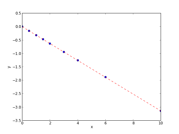
The idea here is to formulate a set of linear equations that is easy to solve. We can express the equations in terms of our unknown fitting parameters $p_i$ as:

x1^0*p0 + x1*p1 = y1
x2^0*p0 + x2*p1 = y2
x3^0*p0 + x3*p1 = y3
etc...

Which we write in matrix form as $A p = y$ where $A$ is a matrix of column vectors, e.g. [1, x_i]. $A$ is not a square matrix, so we cannot solve it as written. Instead, we form $A^T A p = A^T y$ and solve that set of equations.

import numpy as np
x = np.array([0, 0.5, 1, 1.5, 2.0, 3.0, 4.0, 6.0, 10])
y = np.array([0, -0.157, -0.315, -0.472, -0.629, -0.942, -1.255, -1.884, -3.147])

A = np.column_stack([x**0, x])

M = np.dot(A.T, A)
b = np.dot(A.T, y)

i1, slope1 = np.dot(np.linalg.inv(M), b)
i2, slope2 = np.linalg.solve(M, b) # an alternative approach.

print i1, slope1
print i2, slope2

# plot data and fit
import matplotlib.pyplot as plt

plt.plot(x, y, 'bo')
plt.plot(x, np.dot(A, [i1, slope1]), 'r--')
plt.xlabel('x')
plt.ylabel('y')
plt.savefig('images/la-line-fit.png')

0.00062457337884 -0.3145221843
0.00062457337884 -0.3145221843

This method can be readily extended to fitting any polynomial model, or other linear model that is fit in a least squares sense. This method does not provide confidence intervals.

org-mode source

Discuss on Twitter

« Previous Page