Line integrals in Python with autograd

| categories: autograd, integration, python | tags:

Table of Contents

A line integral is an integral of a function along a curve in space. We usually represent the curve by a parametric equation, e.g. \(\mathbf{r}(t) = [x(t), y(t), z(t)] = x(t)\mathbf{i} + y(t)\mathbf{j} + z(t)\mathbf{k}\). So, in general the curve will be a vector function, and the function we want to integrate will also be a vector function.

Then, we can write the line integral definition as:

\(\int_C \mathbf{F(r)}\cdot d\mathbf{r} = \int_a^b \mathbf{F}({\mathbf{r}(t)) \cdot \mathbf{r'}(t) dt\) where \(\mathbf{r'}(t) = \frac{d\mathbf{r}}{dt}\). This integrand is a scalar function, because of the dot product.

The following examples are adapted from Chapter 10 in Advanced Engineering Mathematics by Kreysig.

The first example is the evaluation of a line integral in the plane. We want to evaluate the integral of \(\mathbf{F(r)}=[-y, -xy]\) on the curve \(\mathbf{r(t)}=[-sin(t), cos(t)]\) from t=0 to t = π/2. The answer in the book is given as 0.4521. Here we evaluate this numerically, using autograd for the relevant derivative. Since the curve has multiple outputs, we have to use the jacobian function to get the derivatives. After that, it is a simple bit of matrix multiplication, and a call to the quad function.

import autograd.numpy as np
from autograd import jacobian
from scipy.integrate import quad

def F(X):
    x, y = X
    return -y, -x * y

def r(t):
    return np.array([-np.sin(t), np.cos(t)])

drdt = jacobian(r)

def integrand(t):
    return F(r(t)) @ drdt(t)

I, e = quad(integrand, 0.0, np.pi / 2)
print(f'The integral is {I:1.4f}.')
The integral is 0.4521.


We get the same result as the analytical solution.

The next example is in three dimensions. Find the line integral along \(\mathbf{r}(t)=[cos(t), sin(t), 3t]\) of the function \(\mathbf{F(r)}=[z, x, y]\) from t=0 to t=2 π. The solution is given as 21.99.

import autograd.numpy as np
from autograd import elementwise_grad, grad, jacobian

def F(X):
    x, y, z = X
    return [z, x, y]

def C(t):
    return np.array([np.cos(t), np.sin(t), 3 * t])

dCdt = jacobian(C, 0)

def integrand(t):
    return F(C(t)) @ dCdt(t)

I, e = quad(integrand, 0, 2 * np.pi)
print(f'The integral is {I:1.2f}.')
The integral is 21.99.


That is also the same as the analytical solution. Note the real analytical solution was 7 π, which is nearly equivalent to our answer.

7 * np.pi - I
3.552713678800501e-15

As a final example, we consider an alternate form of the line integral. In this form we do not use a dot product, so the integral results in a vector. This doesn't require anything from autograd, but does require us to be somewhat clever in how to do the integrals since quad can only integrate scalar functions. We need to integrate each component of the integrand independently. Here is one approach where we use lambda functions for each component. You could also manually separate the components.

def F(r):
    x, y, z = r
    return x * y, y * z, z

def r(t):
    return np.array([np.cos(t), np.sin(t), 3 * t])

def integrand(t):
    return F(r(t))

[quad(lambda t: integrand(t)[i], 0, 2 * np.pi)[0] for i in [0, 1, 2]]
[-6.9054847581172525e-18, -18.849555921538755, 59.21762640653615]

The analytical solution in this case was given as:

[0, -6 * np.pi, 6 * np.pi**2]
[0, -18.84955592153876, 59.21762640653615]

which is evidently the same as our numerical solution.

Maybe an alternative, but more verbose is this vectorized integrate function. We still make temporary functions for integrating, and the vectorization is essentially like the list comprehension above, but we avoid the lambda functions.

@np.vectorize
def integrate(i):
    def integrand(t):
        return F(r(t))[i]
    I, e = quad(integrand, 0, 2 * np.pi)
    return I

integrate([0, 1, 2])
array([ -6.90548476e-18,  -1.88495559e+01,   5.92176264e+01])

1 Summary

Once again, autograd provides a convenient way to compute function jacobians which make it easy to evaluate line integrals in Python.

Copyright (C) 2018 by John Kitchin. See the License for information about copying.

org-mode source

Org-mode version = 9.1.14

Discuss on Twitter

Adding a GSL integration function to Emacs with a dynamic module

| categories: integration, dynamic-module, emacs | tags:

Here we work out how to run this program: https://www.gnu.org/software/gsl/doc/html/integration.html#adaptive-integration-example in a dynamic module in emacs. The goal is to be able to evaluate \(\int_0^1 x^{-1/2} \log(x) dx\). According to the example page the answer is -4. We will define an integration function that takes at least a function and integration bounds as arguments, and several optional arguments to specify tolerances and limits. In other words we want to evaluate integrals of the form:

\(\int_a^b f(x; params) dx\)

I want that to happen in an elisp function with a signature like:

(gsl-integration-qags (lambda (x params) body) a b &optional params epsabs epsrel limit)

And that function will return a list containing (result error-estimate). Here is the C-code that makes this happen. It is more complex that the last example, and only compiles with gcc that allows nested functions. I don't know how to write this without that feature. This is more complex also because you have to create a workspace to do the integration inside the function that does the integration. The C-module also has extra code in it to allow for optional arguments.

#include <gsl/gsl_integration.h>
#include "emacs-module.h"

int plugin_is_GPL_compatible;

static emacs_value F_gsl_integrate (emacs_env *env, ptrdiff_t nargs, emacs_value args[], void *data)
{
  // nested function - only supported as an extension in gcc
  double f (double x, void *params) 
  {
    emacs_value fn = args[0];  // function we will integrate
    emacs_value x2[] = { env->make_float(env, x), params };
    emacs_value y = env->funcall(env, fn, 2, &x2);   
    
    return env->extract_float (env, y);
  }

  double a = env->extract_float (env, args[1]);
  double b = env->extract_float (env, args[2]);

  // default values for optional arguments
  double epsabs = 0.0;
  double epsrel = 1e-7;
  size_t limit = 1000;
  double result, error; 

  // Here is how I handle the optional arguments
  // (gsl-integrate func a b params epsabs epsrel limit)
  gsl_function F;
  F.function = &f;
  if (nargs >= 4) {F.params = args[3];}
  if (nargs >= 5 && env->is_not_nil(env, args[4])) {epsabs = env->extract_float(env, args[4]);}
  if (nargs >= 6 && env->is_not_nil(env, args[5])) {epsrel = env->extract_float(env, args[5]);}
  if (nargs >= 7 && env->is_not_nil(env, args[6])) {limit = env->extract_integer(env, args[6]);}

  gsl_integration_workspace * w = gsl_integration_workspace_alloc (limit);

  gsl_integration_qags (&F, // gsl_function pointer
                        a, // lower integration bound
                        b, // upper integration bound
                        epsabs, // absolute error tolerance
                        epsrel, // relative error tolerance
                        limit, // max number of subintervals for integration
                        w, // the workspace
                        // pointers to put results and error in
                        &result, &error);

  gsl_integration_workspace_free (w);
    
  // make a list of (result error) to return
  emacs_value Qlist = env->intern(env, "list");
  emacs_value Qresult = env->make_float (env, result);
  emacs_value Qerror = env->make_float (env, error);
  emacs_value list_args[] = { Qresult, Qerror };
  return env->funcall(env, Qlist, 2, list_args);
}

int emacs_module_init(struct emacs_runtime *ert)
{
  emacs_env *env = ert->get_environment(ert);
  
  // Here we create the function.
  emacs_value fset = env->intern(env, "fset");
  emacs_value args[2];
  args[0] = env->intern(env, "gsl-integration-qags"); // symbol to create for function
  // The function we set that symbol to.
  args[1] = env->make_function(env,
                               3, // min nargs
                               7, // max nargs
                               F_gsl_integrate,
                               "(gsl-integration-qags F A B &optional PARAMS EPSABS EPSREL LIMIT)\n" \
                               "Integrate F(x; params) from A to B.\n" \
                               "F is a function of a single variable and parameters.\n" \
                               "A is the lower bound of integration\n"  \
                               "B is the upper bound of integration.\n" \
                               "Optional parameters:\n"\
                               "PARAMS is a list of params to pass to F.\n" \
                               "EPSABS is a float (default 0.0) and is the absolute error tolerance.\n" \
                               "EPSREL is a float (default 1e-7) and is the relative error tolerance.\n" \
                               "LIMIT is the maximum number of subintervals for the integration (default 1000).\n" \
                               "Returns (list result error-estimate).\n" \
                               "See https://www.gnu.org/software/gsl/manual/html_node/QAGS-adaptive-integration-with-singularities.html.",
                               0);
  // This is basically (fset 'gsl-integration-qags (lambda func))
  env->funcall(env, fset, 2, args);
  
  // This is what allows the shared library to provide a feature 
  emacs_value provide = env->intern(env, "provide");
  emacs_value provide_args[] = { env->intern(env, "gsl-integration") };
  env->funcall(env, provide, 1, provide_args);
  
  return 0;
}

Building this was moderately tricky. It appears the first gcc on my path uses clang which does not support nested functions in C. I don't know enough C to figure out how to do this without a nested function though, since the function has to be defined at run-time based on the emacs env and args. gcc does support inline functions, so the code below uses a gcc that does compile it.

rm -f gsl-integration.so gsl-integration.o
/usr/local/Cellar/gcc/6.1.0/bin/gcc-6 -Wall -I/usr/local/include -fPIC -c gsl-integration.c
/usr/local/Cellar/gcc/6.1.0/bin/gcc-6  -shared -L/usr/local/include -lgsl -o gsl-integration.so gsl-integration.o

Now we add this directory to our path since it is not on it and require our new module.

(add-to-list 'load-path "/Users/jkitchin/vc/blogofile-jkitchin.github.com/_blog/dynamic-module/")
(require 'gsl-integration)
gsl-integration

Let us see our new function in action. We evaluate \(\int_0^1 x^{-1/2} \log(x) dx\). According to the example page the answer is -4. Here is an example where we ignore the parameters. You have to be careful; Emacs sometimes segfaults and crashes if you use an integer or float argument when it expects the other type.

(gsl-integration-qags (lambda (x params) (/ (log x) (sqrt x))) 0.0 1.0)
-4.000000000000085 1.354472090042691e-13

Here are some optional arguments.

(gsl-integration-qags (lambda (x params) (/ (log x) (sqrt x))) 0.0 1.0 nil nil 0.01)
-4.000000000000075 0.019526557540360034

Nice, with a larger epsrel argument we get a larger error. Note the arguments are positional, so we have to include them all just to set the epsrel argument. How about an easier example with parameters that we actually use. Here we integrate a constant, and set the value of the constant from the params arg. The integral should be the area of a rectangle of length 1 and width of the param we use.

(list
 (gsl-integration-qags (lambda (x params) (first params)) 0.0 1.0 '(1.0))
 (gsl-integration-qags (lambda (x params) (first params)) 0.0 1.0 '(0.5)))
1.0 1.1102230246251565e-14
0.5 5.551115123125783e-15

Wow! It actually works!!! That was harder won success than usual for me. I am claiming victory for now and leaving the following notes to future me:

  1. It would be nice to have optional keyword arguments. This would take some handling of the arguments beyond what I know how to do for now, unless it is possible to pull in something like plist-get the way we pull in fset, provide and list in this example.
  2. Error checking on types would be helpful. It is not good for Emacs to crash because 0 is not 0.0!
  3. In numpy there is often a feature to get full_output. Here, the workspace created in the function has more information available in a struct that might be helpful to have access to at times. It seems like it might be possible to get that here too.

Copyright (C) 2017 by John Kitchin. See the License for information about copying.

org-mode source

Org-mode version = 9.0.7

Discuss on Twitter

Numerical Simpsons rule

| categories: integration, math | tags:

A more accurate numerical integration than the trapezoid method is Simpson's rule. The syntax is similar to trapz, but the method is in scipy.integrate.

import numpy as np
from scipy.integrate import simps, romb

a = 0.0; b = np.pi / 4.0;
N = 10  # this is the number of intervals

x = np.linspace(a, b, N)
y = np.cos(x)

t = np.trapz(y, x)
s = simps(y, x)
a = np.sin(b) - np.sin(a)

print
print 'trapz = {0} ({1:%} error)'.format(t, (t - a)/a)
print 'simps = {0} ({1:%} error)'.format(s, (s - a)/a)
print 'analy = {0}'.format(a)
>>> >>> >>> >>> >>> >>> >>> >>> >>> >>> >>> >>>
trapz = 0.70665798038 (-0.063470% error)
simps = 0.707058914216 (-0.006769% error)
analy = 0.707106781187

You can see the Simpson's method is more accurate than the trapezoid method.

Copyright (C) 2013 by John Kitchin. See the License for information about copying.

org-mode source

Discuss on Twitter

Integrating the Fermi distribution to compute entropy

| categories: gotcha, integration, dft | tags:

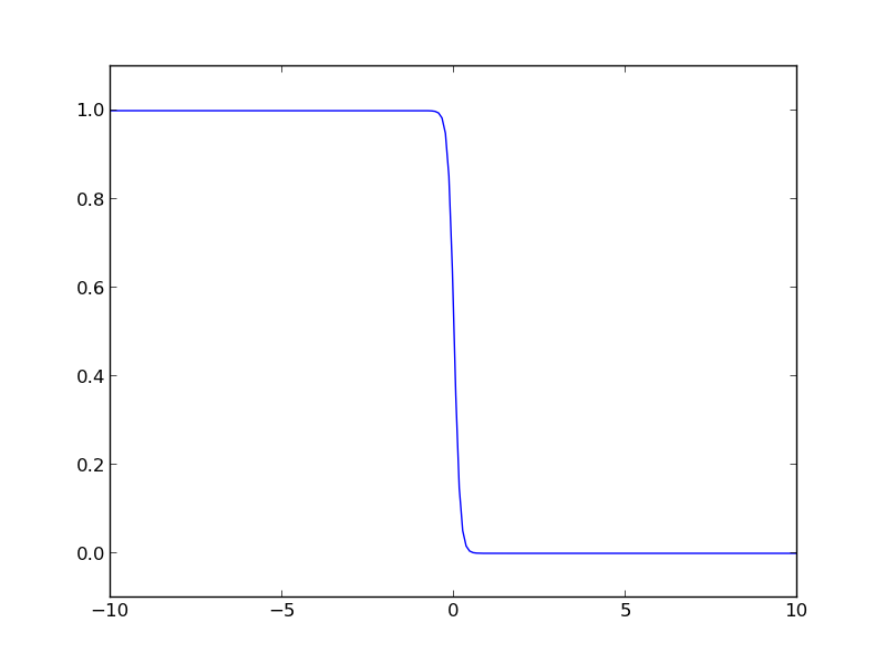
The Fermi distribution is defined by \(f(\epsilon) = \frac{1}{e^{(\epsilon - \mu)/(k T)} + 1}\). This function describes the occupation of energy levels at temperatures above absolute zero. We use this function to compute electronic entropy in a metal, which contains an integral of \(\int n(\epsilon) (f \ln f + (1 - f) \ln (1-f)) d\epsilon\), where \(n(\epsilon)\) is the electronic density of states. Here we plot the Fermi distribution function. It shows that well below the Fermi level the states are fully occupied, and well above the Fermi level, they are unoccupied. Near the Fermi level, the states go from occupied to unoccupied smoothly.

import numpy as np
import matplotlib.pyplot as plt

mu = 0
k = 8.6e-5
T = 1000

def f(e):
    return 1.0 / (np.exp((e - mu)/(k*T)) + 1)

espan = np.linspace(-10, 10, 200)
plt.plot(espan, f(espan))
plt.ylim([-0.1, 1.1])
plt.savefig('images/fermi-entropy-integrand-1.png')

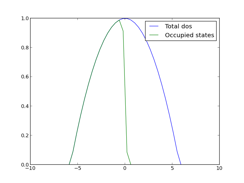
Let us consider a simple density of states function, just a parabola. This could represent a s-band for example. We will use this function to explore the integral.

import numpy as np
import matplotlib.pyplot as plt

mu = 0
k = 8.6e-5
T = 1000

def f(e):
    return 1.0 / (np.exp((e - mu)/(k*T)) + 1)

def dos(e):
    d = (np.ones(e.shape) - 0.03 * e**2) 
    return d * (d > 0)
espan = np.linspace(-10, 10)

plt.plot(espan, dos(espan), label='Total dos')
plt.plot(espan, f(espan) * dos(espan), label='Occupied states')
plt.legend(loc='best')
plt.savefig('images/fermi-entropy-integrand-2.png')

Now, we consider the integral to compute the electronic entropy. The entropy is proportional to this integral.

\( \int n(\epsilon) (f \ln f + (1 - f) \ln (1-f)) d\epsilon \)

It looks straightforward to compute, but it turns out there is a wrinkle. Evaluating the integrand leads to nan elements because the ln(0) is -∞.

import numpy as np
mu = 0
k = 8.6e-5
T = 100

def fermi(e):
    return 1.0 / (np.exp((e - mu)/(k*T)) + 1)

espan = np.array([-20, -10, -5, 0.0, 5, 10])
f = fermi(espan)

print f * np.log(f)
print (1 - f) * np.log(1 - f)
[  0.00000000e+000   0.00000000e+000   0.00000000e+000  -3.46573590e-001
  -1.85216532e-250               nan]
[        nan         nan         nan -0.34657359  0.          0.        ]

In this case, these nan elements should be equal to zero (x ln(x) goes to zero as x goes to zero). So, we can just ignore those elements in the integral. Here is how to do that.

import numpy as np
import matplotlib.pyplot as plt

mu = 0
k = 8.6e-5
T = 1000

def fermi(e):
    return 1.0 / (np.exp((e - mu)/(k*T)) + 1)

def dos(e):
    d = (np.ones(e.shape) - 0.03 * e**2) 
    return d * (d > 0)

espan = np.linspace(-20, 10)
f = fermi(espan)
n = dos(espan)

g = n * (f * np.log(f) + (1 - f) * np.log(1 - f))

print np.trapz(espan, g) # nan because of the nan in the g vector
print g

plt.plot(espan, g)
plt.savefig('images/fermi-entropy-integrand-3.png')

# find the elements that are not nan
ind = np.logical_not(np.isnan(g))

# evaluate the integrand for only those points
print np.trapz(espan[ind], g[ind])
nan
[             nan              nan              nan              nan
              nan              nan              nan              nan
              nan              nan              nan              nan
              nan              nan              nan              nan
              nan              nan              nan              nan
              nan              nan              nan              nan
              nan              nan              nan              nan
  -9.75109643e-14  -1.05987106e-10  -1.04640574e-07  -8.76265644e-05
  -4.92684641e-02  -2.91047740e-01  -7.75652579e-04  -1.00962241e-06
  -1.06972936e-09  -1.00527877e-12  -8.36436686e-16  -6.48930917e-19
  -4.37946336e-22  -2.23285389e-25  -1.88578082e-29   0.00000000e+00
   0.00000000e+00   0.00000000e+00   0.00000000e+00   0.00000000e+00
   0.00000000e+00   0.00000000e+00]
0.208886080897

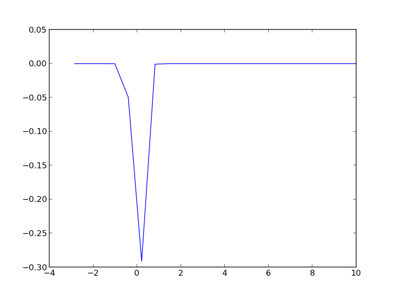
The integrand is pretty well behaved in the figure above. You do not see the full range of the x-axis, because the integrand evaluates to nan for very negative numbers. This causes the trapz function to return nan also. We can solve the problem by only integrating the parts that are not nan. We have to use numpy.logicalnot to get an element-wise array of which elements are not nan. In this example, the integrand is not well sampled, so the area under that curve may not be very accurate.

Copyright (C) 2013 by John Kitchin. See the License for information about copying.

org-mode source

Discuss on Twitter

The trapezoidal method of integration

| categories: integration, math | tags:

Matlab post See http://en.wikipedia.org/wiki/Trapezoidal_rule

$$\int_a^b f(x) dx \approx \frac{1}{2}\displaystyle\sum\limits_{k=1}^N(x_{k+1}-x_k)(f(x_{k+1}) + f(x_k))$$

Let us compute the integral of sin(x) from x=0 to \(\pi\). To approximate the integral, we need to divide the interval from \(a\) to \(b\) into \(N\) intervals. The analytical answer is 2.0.

We will use this example to illustrate the difference in performance between loops and vectorized operations in python.

import numpy as np
import time

a = 0.0; b = np.pi;
N = 1000; # this is the number of intervals

h = (b - a)/N; # this is the width of each interval
x = np.linspace(a, b, N) 
y = np.sin(x); # the sin function is already vectorized

t0 = time.time()
f = 0.0
for k in range(len(x) - 1):
    f += 0.5 * ((x[k+1] - x[k]) * (y[k+1] + y[k]))

tf = time.time() - t0
print 'time elapsed = {0} sec'.format(tf)

print f
>>> >>> >>> >>> >>> >>> >>> >>> >>> >>> >>> ... ... >>> >>> time elapsed = 0.0780000686646 sec
>>> 1.99999835177
t0 = time.time()
Xk = x[1:-1] - x[0:-2] # vectorized version of (x[k+1] - x[k])
Yk = y[1:-1] + y[0:-2] # vectorized version of (y[k+1] + y[k])

f = 0.5 * np.sum(Xk * Yk) # vectorized version of the loop above
tf = time.time() - t0
print 'time elapsed = {0} sec'.format(tf)

print f
>>> >>> >>> >>> >>> time elapsed = 0.077999830246 sec
>>> 1.99999340709

In the last example, there may be loop buried in the sum command. Let us do one final method, using linear algebra, in a single line. The key to understanding this is to recognize the sum is just the result of a dot product of the x differences and y sums.

t0 = time.time()
f = 0.5 * np.dot(Xk, Yk)
tf = time.time() - t0
print 'time elapsed = {0} sec'.format(tf)

print f
>>> >>> time elapsed = 0.0310001373291 sec
>>> 1.99999340709

The loop method is straightforward to code, and looks alot like the formula that defines the trapezoid method. the vectorized methods are not as easy to read, and take fewer lines of code to write. However, the vectorized methods are much faster than the loop, so the loss of readability could be worth it for very large problems.

The times here are considerably slower than in Matlab. I am not sure if that is a totally fair comparison. Here I am running python through emacs, which may result in slower performance. I also used a very crude way of timing the performance which lumps some system performance in too.

Copyright (C) 2013 by John Kitchin. See the License for information about copying.

org-mode source

Discuss on Twitter
Next Page ยป