The Kitchin Research Group

In this post I explored using automatic differentiation to compute how the compressibility of a gas defined by the van der Waal equation varies with the reduced pressure. In that example we had an explicit function of the pressure as a function of the volume and temperature, and we could derive a differential equation that defines the variation we were interested in.

I thought we should be able to derive the differential equation more directly, still using automatic differentiation and we explore that idea here. The general strategy to compute the compressibility as a function of pressure is to integrate \(dV / dP_r\) over a range of \(P_r\) to get the molar volume as a function of \(P_r\), and then to directly compute the compressibility from \(Z = PV/(RT)\).

To use this approach we need to get \(dV / dP_r\) from the van der Waal equation. Previously, we derived this in a round about way from the explicit form of the van der Waal equation. Here, we follow the work in this post to get the derivative from the implicit form of the van der Waal equation:

\(f(V, P_r, T_r) = \frac{R Tr * Tc}{V - b} - \frac{a}{V^2} - P_r Pc = 0\)

Based on the work in this post, we can get

\(dV/dP_r = (-df/dP_r) / (df/dV)\)

and the two derivatives on the right can be found easily by automatic differentiation. First, we express the van der Waal equation in implicit form, with the variables as \(V, P_r, T_r\). Only two of those variables are independent; if you define two of them you can compute the third one using a tool like fsolve.

R = 0.08206
Pc = 72.9
Tc = 304.2

a = 27 * R**2 * Tc**2 / (Pc * 64)
b = R * Tc / (8 * Pc)

Tr = 1.1  # Constant for this example

def f(V, Pr, Tr):
    return R * Tr * Tc / (V - b) - a / V**2 - Pr * Pc

Now, if we want to know how does the volume vary with \(P_r\), we need to derive the derivative \(dV/dP_r\), and then integrate it. Here we use autograd to define the derivatives, and then we define a function that uses them. Note the arguments in the function dVdPr are in an order that anticipates we want to integrate it in solve_ivp, to get a function \(V(P_r)\).

from autograd import grad

dfdPr = grad(f, 1)  # derivative of f with respect to arg at index=1: Pr
dfdV = grad(f, 0)  # derivative of f with respect to arg at index=0: V

def dVdPr(Pr, V):
    return -dfdPr(V, Pr, Tr) / dfdV(V, Pr, Tr)  # Tr is a constant in here

Now, we need an initial condition to start the integration from. We want the volume at \(P_r=0.1\). We have to use fsolve for this, or some other method that tells you want is the volume at \(P_r=0.1\). We can pass the values of \(P_r\) and \(T_R\) as arguments to our implicit function. Since \(V\) is the first argument, we can directly solve our implicit function. Otherwise you would have to define a helper objective function to use with fsolve.

from scipy.optimize import fsolve

V0, = fsolve(f, 3.5, args=(0.1, 1.1))
V0

3.6764763125625435

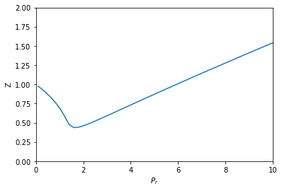
Finally, we are ready to integrate the ODE, and plot the solution.

import numpy as np
from scipy.integrate import solve_ivp

Pr_span = (0.1, 10)
Pr_eval, h = np.linspace(*Pr_span, retstep=True)

sol = solve_ivp(dVdPr, Pr_span, (V0,), max_step=h)
print(sol.message)

%matplotlib inline
import matplotlib.pyplot as plt

Pr = sol.t  # the P_r steps used in the solution
V = sol.y[0]  # V(P_r) from the solution

Z = Pr * Pc * V / (R * Tr * Tc)  # Compressibility Z(P_r)

plt.plot(Pr, Z)
plt.xlabel('$P_r$')
plt.ylabel('Z')
plt.xlim([0, 10])
plt.ylim([0, 2])

The solver successfully reached the end of the integration interval.

(0, 2)

That is the same result as we got before.

Copyright (C) 2018 by John Kitchin. See the License for information about copying.

org-mode source

Org-mode version = 9.1.13