Estimating where two functions intersect using data

Posted July 04, 2013 at 02:38 PM | categories: data analysis | tags:

Updated July 07, 2013 at 09:01 AM

Suppose we have two functions described by this data:

T(K)	E1	E2
300	-208	-218
400	-212	-221
500	-215	-220
600	-218	-222
700	-220	-222
800	-223	-224
900	-227	-225
1000	-229	-227
1100	-233	-228
1200	-235	-227
1300	-240	-229

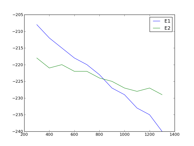
We want to determine the temperature at which they intersect, and more importantly what the uncertainty on the intersection is. There is noise in the data, which means there is uncertainty in any function that could be fit to it, and that uncertainty would propagate to the intersection. Let us examine the data.

import matplotlib.pyplot as plt

T = [x[0] for x in data]
E1 = [x[1] for x in data]
E2 = [x[2] for x in data]

plt.plot(T, E1, T, E2)
plt.legend(['E1', 'E2'])
plt.savefig('images/intersection-0.png')

Our strategy is going to be to fit functions to each data set, and get the confidence intervals on the parameters of the fit. Then, we will solve the equations to find where they are equal to each other and propagate the uncertainties in the parameters to the answer.

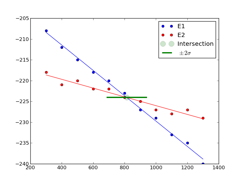
These functions look approximately linear, so we will fit lines to each function. We use the regress function in pycse to get the uncertainties on the fits. Then, we use the uncertainties package to propagate the uncertainties in the analytical solution to the intersection of two lines.

import numpy as np
from pycse import regress
import matplotlib.pyplot as plt
import uncertainties as u

T = np.array([x[0] for x in data])
E1 = np.array([x[1] for x in data])
E2 = np.array([x[2] for x in data])

# columns of the x-values for a line: constant, T
A = np.column_stack([T**0, T])

p1, pint1, se1 = regress(A, E1, alpha=0.05)

p2, pint2, se2 = regress(A, E2, alpha=0.05)

# Now we have two lines: y1 = m1*T + b1 and y2 = m2*T + b2
# they intersect at m1*T + b1 = m2*T + b2
# or at T = (b2 - b1) / (m1 - m2)
b1 = u.ufloat((p1[0], se1[0]))
m1 = u.ufloat((p1[1], se1[1]))

b2 = u.ufloat((p2[0], se2[0]))
m2 = u.ufloat((p2[1], se2[1]))

T_intersection = (b2 - b1) / (m1 - m2)
print T_intersection

# plot the data, the fits and the intersection and \pm 2 \sigma.
plt.plot(T, E1, 'bo ', label='E1')
plt.plot(T, np.dot(A,p1), 'b-')
plt.plot(T, E2, 'ro ', label='E2')
plt.plot(T, np.dot(A,p2), 'r-')

plt.plot(T_intersection.nominal_value,
        (b1 + m1*T_intersection).nominal_value, 'go',
        ms=13, alpha=0.2, label='Intersection')
plt.plot([T_intersection.nominal_value - 2*T_intersection.std_dev(),
          T_intersection.nominal_value + 2*T_intersection.std_dev()],
         [(b1 + m1*T_intersection).nominal_value, 
          (b1 + m1*T_intersection).nominal_value],
         'g-', lw=3, label='$\pm 2 \sigma$')
       
plt.legend(loc='best')
plt.savefig('images/intersection-1.png')

813.698630137+/-62.407180552

You can see there is a substantial uncertainty in the temperature at approximately the 90% confidence level (± 2 σ).

Update 7-7-2013

After a suggestion from Prateek, here we subtract the two data sets, fit a line to that data, and then use fsolve to find the zero. We wrap fsolve in the uncertainties package to directly get the uncertainty on the root.

import numpy as np
from pycse import regress
import matplotlib.pyplot as plt
import uncertainties as u
from scipy.optimize import fsolve


T = np.array([x[0] for x in data])
E1 = np.array([x[1] for x in data])
E2 = np.array([x[2] for x in data])

E = E1 - E2

# columns of the x-values for a line: constant, T
A = np.column_stack([T**0, T])

p, pint, se = regress(A, E, alpha=0.05)

b = u.ufloat((p[0], se[0]))
m = u.ufloat((p[1], se[1]))

@u.wrap
def f(b, m):
    X, = fsolve(lambda x: b + m * x, 800)
    return X

print f(b, m)

813.698630137+/-54.0386903923

Interesting that this uncertainty is a little smaller than the previously computed uncertainty. Here you can see we have to wrap the function in a peculiar way. The function must return a single float number, and take arguments with uncertainty. We define the polynomial fit (a line in this case) in a lambda function inside the function. It works ok.

org-mode source

The Kitchin Research Group

Chemical Engineering at Carnegie Mellon University

Estimating where two functions intersect using data