Estimating uncertainties in equations of state
Posted July 04, 2013 at 03:21 PM | categories: uncategorized | tags:
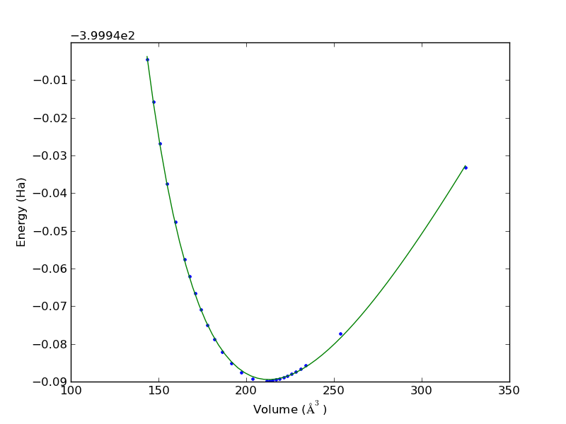
We often use DFT to calculate the energy of a unit cell as a function of volume. Then, we fit an equation of state to the data to estimate the volume that minimizes the total energy, and the bulk modulus of the material. 10.1016/j.comphys.2003.12.001
| volume | energy |
|---|---|
| 324.85990899 | -399.9731688470 |
| 253.43999457 | -400.0172393178 |
| 234.03826687 | -400.0256270548 |
| 231.12159387 | -400.0265690700 |
| 228.40609504 | -400.0273551120 |
| 225.86490337 | -400.0280030862 |
| 223.47556626 | -400.0285313450 |
| 221.21992353 | -400.0289534593 |
| 219.08319566 | -400.0292800709 |
| 217.05369547 | -400.0295224970 |
| 215.12089909 | -400.0296863867 |
| 213.27525144 | -400.0297809256 |
| 211.51060823 | -400.0298110000 |
| 203.66743321 | -400.0291665573 |
| 197.07888649 | -400.0275017142 |
| 191.39717952 | -400.0250998136 |
| 186.40163591 | -400.0221371852 |
| 181.94435510 | -400.0187369863 |
| 177.92077043 | -400.0149820198 |
| 174.25380090 | -400.0109367042 |
| 170.88582166 | -400.0066495100 |
| 167.76711189 | -400.0021478258 |
| 164.87096104 | -399.9974753449 |
| 159.62553397 | -399.9876885136 |
| 154.97005460 | -399.9774175487 |
| 150.78475335 | -399.9667603369 |
| 146.97722201 | -399.9557686286 |
| 143.49380641 | -399.9445262604 |
import numpy as np
import matplotlib.pyplot as plt
from pycse import nlinfit

# data
V = np.array([row[0] for row in data])
E = np.array([row[1] for row in data])

plt.plot(V, E, '.')
plt.xlabel('Volume ($\AA^3$)')
plt.ylabel('Energy (Ha)')

def Murnaghan(vol, E0, B0, BP, V0):
    '''
    given a vector of parameters and volumes, return a vector of energies.
    equation From PRB 28,5480 (1983)
    '''

    E = E0 + B0*vol/BP*(((V0/vol)**BP)/(BP-1)+1) - V0*B0/(BP-1.)

    return E

guess = [-400, 0.5, 2, 210]
pars, pint, SE = nlinfit(Murnaghan, V, E, guess, alpha=0.05)
E0, B0, BP, V0 = pint

Vfit = np.linspace(V.min(), V.max())
plt.plot(Vfit, Murnaghan(Vfit, *pars))
plt.savefig('images/eos-uncertainty.png')

print '95% confidence intervals'
print 'V0 = {0} bohr**3'.format(V0)
print 'E0 = {0} Ha'.format(E0)
print 'B0 = {0} GPA'.format([x * 29421.010901602753 for x in B0])
95% confidence intervals
V0 = [212.27788154532402, 213.27897592511891] bohr**3
E0 = [-400.0297027767362, -400.02922937100408] Ha
B0 = [108.62283904402159, 111.20447706313001] GPA

You can see the fit is not perfect, and there is corresponding uncertainty in the estimated parameters. A nice feature of the Murnaghan equation of state is that the parameters are directly the quantities of interest, so the uncertainties are directly calculated here. For other models, e.g. a polynomial fit, you would have to propagate the errors in the parameters to the properties.
Copyright (C) 2013 by John Kitchin. See the License for information about copying.