The Kitchin Research Group

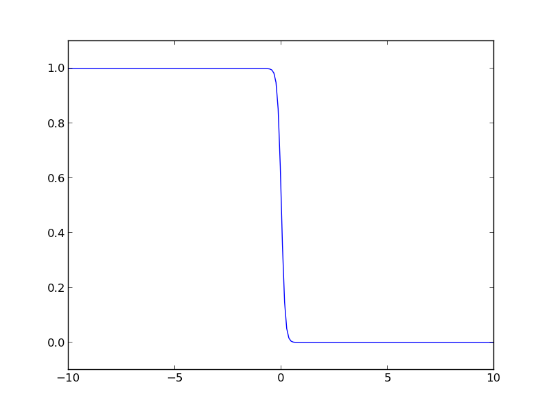
The Fermi distribution is defined by \(f(\epsilon) = \frac{1}{e^{(\epsilon - \mu)/(k T)} + 1}\). This function describes the occupation of energy levels at temperatures above absolute zero. We use this function to compute electronic entropy in a metal, which contains an integral of \(\int n(\epsilon) (f \ln f + (1 - f) \ln (1-f)) d\epsilon\), where \(n(\epsilon)\) is the electronic density of states. Here we plot the Fermi distribution function. It shows that well below the Fermi level the states are fully occupied, and well above the Fermi level, they are unoccupied. Near the Fermi level, the states go from occupied to unoccupied smoothly.

import numpy as np
import matplotlib.pyplot as plt

mu = 0
k = 8.6e-5
T = 1000

def f(e):
    return 1.0 / (np.exp((e - mu)/(k*T)) + 1)

espan = np.linspace(-10, 10, 200)
plt.plot(espan, f(espan))
plt.ylim([-0.1, 1.1])
plt.savefig('images/fermi-entropy-integrand-1.png')

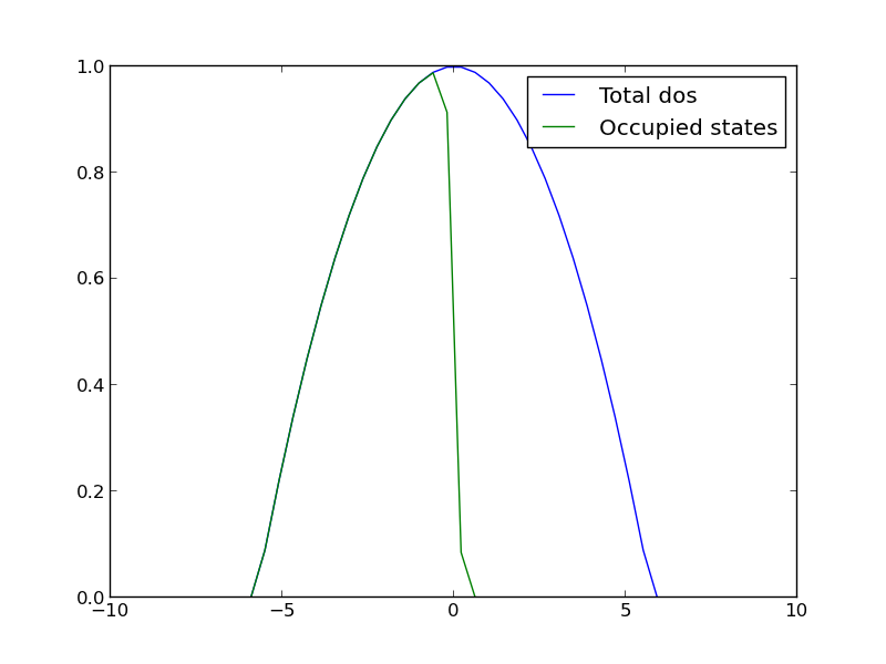
Let us consider a simple density of states function, just a parabola. This could represent a s-band for example. We will use this function to explore the integral.

import numpy as np
import matplotlib.pyplot as plt

mu = 0
k = 8.6e-5
T = 1000

def f(e):
    return 1.0 / (np.exp((e - mu)/(k*T)) + 1)

def dos(e):
    d = (np.ones(e.shape) - 0.03 * e**2) 
    return d * (d > 0)
espan = np.linspace(-10, 10)

plt.plot(espan, dos(espan), label='Total dos')
plt.plot(espan, f(espan) * dos(espan), label='Occupied states')
plt.legend(loc='best')
plt.savefig('images/fermi-entropy-integrand-2.png')

Now, we consider the integral to compute the electronic entropy. The entropy is proportional to this integral.

\( \int n(\epsilon) (f \ln f + (1 - f) \ln (1-f)) d\epsilon \)

It looks straightforward to compute, but it turns out there is a wrinkle. Evaluating the integrand leads to nan elements because the ln(0) is -∞.

import numpy as np
mu = 0
k = 8.6e-5
T = 100

def fermi(e):
    return 1.0 / (np.exp((e - mu)/(k*T)) + 1)

espan = np.array([-20, -10, -5, 0.0, 5, 10])
f = fermi(espan)

print f * np.log(f)
print (1 - f) * np.log(1 - f)

[  0.00000000e+000   0.00000000e+000   0.00000000e+000  -3.46573590e-001
  -1.85216532e-250               nan]
[        nan         nan         nan -0.34657359  0.          0.        ]

In this case, these nan elements should be equal to zero (x ln(x) goes to zero as x goes to zero). So, we can just ignore those elements in the integral. Here is how to do that.

import numpy as np
import matplotlib.pyplot as plt

mu = 0
k = 8.6e-5
T = 1000

def fermi(e):
    return 1.0 / (np.exp((e - mu)/(k*T)) + 1)

def dos(e):
    d = (np.ones(e.shape) - 0.03 * e**2) 
    return d * (d > 0)

espan = np.linspace(-20, 10)
f = fermi(espan)
n = dos(espan)

g = n * (f * np.log(f) + (1 - f) * np.log(1 - f))

print np.trapz(espan, g) # nan because of the nan in the g vector
print g

plt.plot(espan, g)
plt.savefig('images/fermi-entropy-integrand-3.png')

# find the elements that are not nan
ind = np.logical_not(np.isnan(g))

# evaluate the integrand for only those points
print np.trapz(espan[ind], g[ind])

nan
[             nan              nan              nan              nan
              nan              nan              nan              nan
              nan              nan              nan              nan
              nan              nan              nan              nan
              nan              nan              nan              nan
              nan              nan              nan              nan
              nan              nan              nan              nan
  -9.75109643e-14  -1.05987106e-10  -1.04640574e-07  -8.76265644e-05
  -4.92684641e-02  -2.91047740e-01  -7.75652579e-04  -1.00962241e-06
  -1.06972936e-09  -1.00527877e-12  -8.36436686e-16  -6.48930917e-19
  -4.37946336e-22  -2.23285389e-25  -1.88578082e-29   0.00000000e+00
   0.00000000e+00   0.00000000e+00   0.00000000e+00   0.00000000e+00
   0.00000000e+00   0.00000000e+00]
0.208886080897

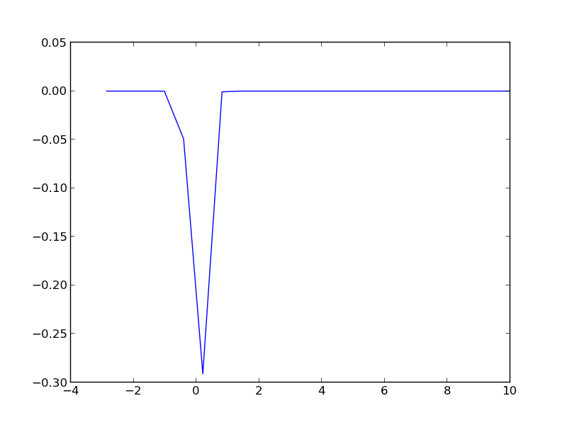
The integrand is pretty well behaved in the figure above. You do not see the full range of the x-axis, because the integrand evaluates to nan for very negative numbers. This causes the trapz function to return nan also. We can solve the problem by only integrating the parts that are not nan. We have to use numpy.logical_not to get an element-wise array of which elements are not nan. In this example, the integrand is not well sampled, so the area under that curve may not be very accurate.

Copyright (C) 2013 by John Kitchin. See the License for information about copying.

org-mode source