The Kitchin Research Group

Matlab post

For steady state heat conduction the temperature distribution in one-dimension is governed by the Laplace equation:

$$ \nabla^2 T = 0$$

with boundary conditions that at \(T(x=a) = T_A\) and \(T(x=L) = T_B\).

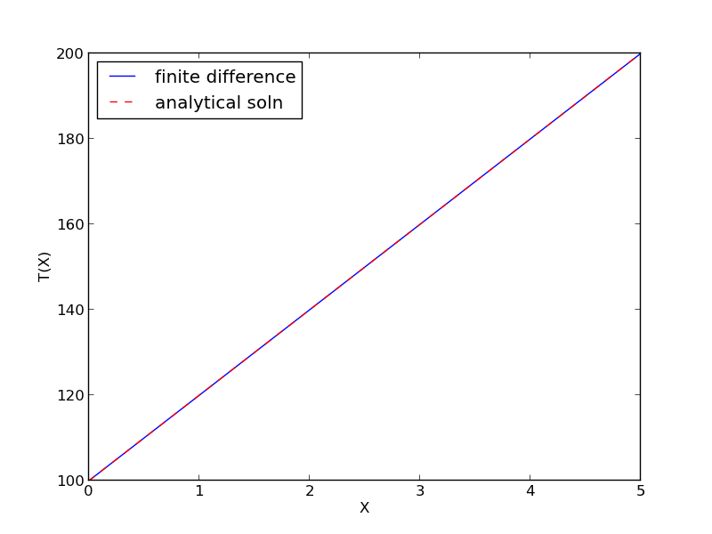
The analytical solution is not difficult here: \(T = T_A-\frac{T_A-T_B}{L}x\), but we will solve this by finite differences.

For this problem, lets consider a slab that is defined by x=0 to x=L, with \(T(x=0) = 100\), and \(T(x=L) = 200\). We want to find the function T(x) inside the slab.

We approximate the second derivative by finite differences as

\( f''(x) \approx \frac{f(x-h) - 2 f(x) + f(x+h)}{h^2} \)

Since the second derivative in this case is equal to zero, we have at each discretized node \(0 = T_{i-1} - 2 T_i + T_{i+1}\). We know the values of \(T_{x=0} = \alpha\) and \(T_{x=L} = \beta\).

\[A = \left [ \begin{array}{ccccc} % -2 & 1 & 0 & 0 & 0 \\ 1 & -2& 1 & 0 & 0 \\ 0 & \ddots & \ddots & \ddots & 0 \\ 0 & 0 & 1 & -2 & 1 \\ 0 & 0 & 0 & 1 & -2 \end{array} \right ] \]

\[ x = \left [ \begin{array}{c} T_1 \\ \vdots \\ T_N \end{array} \right ] \]

\[ b = \left [ \begin{array}{c} -T(x=0) \\ 0 \\ \vdots \\ 0 \\ -T(x=L) \end{array} \right] \]

These are linear equations in the unknowns \(x\) that we can easily solve. Here, we evaluate the solution.

import numpy as np

#we use the notation T(x1) = alpha and T(x2) = beta
x1 = 0; alpha = 100
x2 = 5; beta = 200

npoints = 100

# preallocate and shape the b vector and A-matrix
b = np.zeros((npoints, 1));
b[0] = -alpha
b[-1] = -beta

A = np.zeros((npoints, npoints));

#now we populate the A-matrix and b vector elements
for i in range(npoints ):
    for j in range(npoints):
        if j == i: # the diagonal
            A[i,j] = -2
        elif j == i - 1: # left of the diagonal
            A[i,j] = 1
        elif j == i + 1: # right of the diagonal
            A[i,j] = 1
 
# solve the equations A*y = b for Y
Y = np.linalg.solve(A,b)

x = np.linspace(x1, x2, npoints + 2)
y = np.hstack([alpha, Y[:,0], beta])

import matplotlib.pyplot as plt

plt.plot(x, y)

plt.plot(x, alpha + (beta - alpha)/(x2 - x1) * x, 'r--')

plt.xlabel('X')
plt.ylabel('T(X)')
plt.legend(('finite difference', 'analytical soln'), loc='best')
plt.savefig('images/bvp-heat-conduction-1d.png')

Copyright (C) 2013 by John Kitchin. See the License for information about copying.

org-mode source