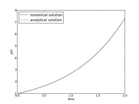
Numerical solution to a simple ode
Posted February 26, 2013 at 09:17 PM | categories: interpolation, ode | tags:
Updated March 23, 2013 at 04:03 PM
Integrate this ordinary differential equation (ode):
$$\frac{dy}{dt} = y(t)$$
over the time span of 0 to 2. The initial condition is y(0) = 1.
to solve this equation, you need to create a function of the form: dydt = f(y, t) and then use one of the odesolvers, e.g. odeint.
import numpy as np
from scipy.integrate import odeint
import matplotlib.pyplot as plt

def fprime(y,t):
    return y

tspan = np.linspace(0, 2)
y0 = 1
ysol = odeint(fprime, y0, tspan)

plt.plot(tspan, ysol, label='numerical solution')
plt.plot(tspan, np.exp(tspan), 'r--', label='analytical solution')
plt.xlabel('time')
plt.ylabel('y(t)')
plt.legend(loc='best')
plt.savefig('images/simple-ode.png')

The numerical and analytical solutions agree.
Now, suppose you want to know at what time is the solution equal to 3? There are several approaches to this, including setting up a solver, or using an event like approach to stop integration at y=3. A simple approach is to use reverse interpolation. We simply reverse the x and y vectors so that y is the independent variable, and we interpolate the corresponding x-value.
import numpy as np
from scipy.integrate import odeint
import matplotlib.pyplot as plt

def fprime(y,t):
    return y

tspan = np.linspace(0, 2)
y0 = 1
ysol = odeint(fprime, y0, tspan)

from scipy.interpolate import interp1d

ip = interp1d(ysol[:,0], tspan) # reverse interpolation
print 'y = 3 at x = {0}'.format(ip(3))
y = 3 at x = 1.09854780564
Copyright (C) 2013 by John Kitchin. See the License for information about copying.