The Kitchin Research Group

Matlab post

adapted from http://www.itl.nist.gov/div898/handbook/pmd/section4/pmd44.htm

In this example, we show some ways to choose which of several models fit data the best. We have data for the total pressure and temperature of a fixed amount of a gas in a tank that was measured over the course of several days. We want to select a model that relates the pressure to the gas temperature.

The data is stored in a text file download PT.txt , with the following structure:

Run          Ambient                            Fitted
 Order  Day  Temperature  Temperature  Pressure    Value    Residual
  1      1      23.820      54.749      225.066   222.920     2.146
...

We need to read the data in, and perform a regression analysis on P vs. T. In python we start counting at 0, so we actually want columns 3 and 4.

import numpy as np
import matplotlib.pyplot as plt

data = np.loadtxt('data/PT.txt', skiprows=2)
T = data[:, 3]
P = data[:, 4]

plt.plot(T, P, 'k.')
plt.xlabel('Temperature')
plt.ylabel('Pressure')
plt.savefig('images/model-selection-1.png')

>>> >>> >>> >>> >>> >>> [<matplotlib.lines.Line2D object at 0x00000000084398D0>]
<matplotlib.text.Text object at 0x000000000841F6A0>
<matplotlib.text.Text object at 0x0000000008423DD8>

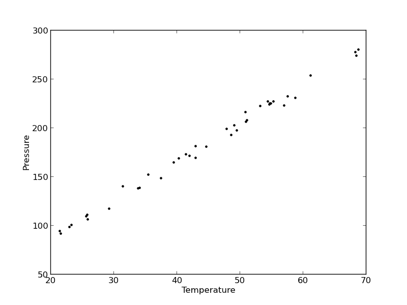
It appears the data is roughly linear, and we know from the ideal gas law that PV = nRT, or P = nR/V*T, which says P should be linearly correlated with V. Note that the temperature data is in degC, not in K, so it is not expected that P=0 at T = 0. We will use linear algebra to compute the line coefficients.

A = np.vstack([T**0, T]).T
b = P

x, res, rank, s = np.linalg.lstsq(A, b)
intercept, slope = x
print 'b, m =', intercept, slope

n = len(b)
k = len(x)

sigma2 = np.sum((b - np.dot(A,x))**2) / (n - k)

C = sigma2 * np.linalg.inv(np.dot(A.T, A))
se = np.sqrt(np.diag(C))

from scipy.stats.distributions import  t
alpha = 0.05

sT = t.ppf(1-alpha/2., n - k) # student T multiplier
CI = sT * se

print 'CI = ',CI
for beta, ci in zip(x, CI):
    print '[{0} {1}]'.format(beta - ci, beta + ci)

>>> >>> >>> >>> b, m = 7.74899739238 3.93014043824
>>> >>> >>> >>> >>> >>> >>> >>> >>> >>> >>> >>> >>> >>> >>> CI =  [ 4.76511545  0.1026405 ]
... ... [2.98388194638 12.5141128384]
[3.82749994079 4.03278093569]

The confidence interval on the intercept is large, but it does not contain zero at the 95% confidence level.

The R^2 value accounts roughly for the fraction of variation in the data that can be described by the model. Hence, a value close to one means nearly all the variations are described by the model, except for random variations.

ybar = np.mean(P)
SStot = np.sum((P - ybar)**2)
SSerr = np.sum((P - np.dot(A, x))**2)
R2 = 1 - SSerr/SStot
print R2

>>> >>> >>> 0.993715411798

plt.figure(); plt.clf()
plt.plot(T, P, 'k.', T, np.dot(A, x), 'b-')
plt.xlabel('Temperature')
plt.ylabel('Pressure')
plt.title('R^2 = {0:1.3f}'.format(R2))
plt.savefig('images/model-selection-2.png')

<matplotlib.figure.Figure object at 0x0000000008423860>
[<matplotlib.lines.Line2D object at 0x00000000085BE780>, <matplotlib.lines.Line2D object at 0x00000000085BE940>]
<matplotlib.text.Text object at 0x0000000008449898>
<matplotlib.text.Text object at 0x000000000844CCF8>
<matplotlib.text.Text object at 0x000000000844ED30>

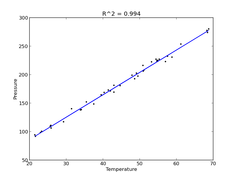
The fit looks good, and R^2 is near one, but is it a good model? There are a few ways to examine this. We want to make sure that there are no systematic trends in the errors between the fit and the data, and we want to make sure there are not hidden correlations with other variables. The residuals are the error between the fit and the data. The residuals should not show any patterns when plotted against any variables, and they do not in this case.

residuals = P - np.dot(A, x)

plt.figure()

f, (ax1, ax2, ax3) = plt.subplots(3)

ax1.plot(T,residuals,'ko')
ax1.set_xlabel('Temperature')


run_order = data[:, 0]
ax2.plot(run_order, residuals,'ko ')
ax2.set_xlabel('run order')

ambientT = data[:, 2]
ax3.plot(ambientT, residuals,'ko')
ax3.set_xlabel('ambient temperature')

plt.tight_layout() # make sure plots do not overlap

plt.savefig('images/model-selection-3.png')

>>> <matplotlib.figure.Figure object at 0x00000000085C21D0>
>>> >>> >>> [<matplotlib.lines.Line2D object at 0x0000000008861CC0>]
<matplotlib.text.Text object at 0x00000000085D3A58>
>>> >>> >>> [<matplotlib.lines.Line2D object at 0x0000000008861E80>]
<matplotlib.text.Text object at 0x00000000085EC5F8>
>>> >>> [<matplotlib.lines.Line2D object at 0x0000000008861C88>]
<matplotlib.text.Text object at 0x0000000008846828>

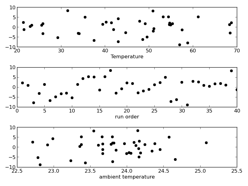
There may be some correlations in the residuals with the run order. That could indicate an experimental source of error.

We assume all the errors are uncorrelated with each other. We can use a lag plot to assess this, where we plot residual[i] vs residual[i-1], i.e. we look for correlations between adjacent residuals. This plot should look random, with no correlations if the model is good.

plt.figure(); plt.clf()
plt.plot(residuals[1:-1], residuals[0:-2],'ko')
plt.xlabel('residual[i]')
plt.ylabel('residual[i-1]')
plt.savefig('images/model-selection-correlated-residuals.png')

<matplotlib.figure.Figure object at 0x000000000886EB00>
[<matplotlib.lines.Line2D object at 0x0000000008A02908>]
<matplotlib.text.Text object at 0x00000000089E8198>
<matplotlib.text.Text object at 0x00000000089EB908>

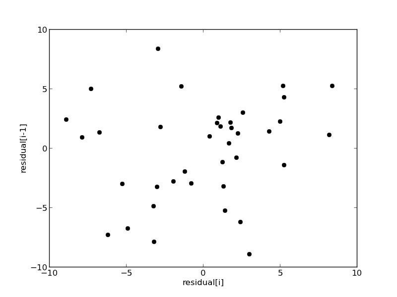
It is hard to argue there is any correlation here.

Lets consider a quadratic model instead.

A = np.vstack([T**0, T, T**2]).T
b = P;

x, res, rank, s = np.linalg.lstsq(A, b)
print x

n = len(b)
k = len(x)

sigma2 = np.sum((b - np.dot(A,x))**2) / (n - k)

C = sigma2 * np.linalg.inv(np.dot(A.T, A))
se = np.sqrt(np.diag(C))

from scipy.stats.distributions import  t
alpha = 0.05

sT = t.ppf(1-alpha/2., n - k) # student T multiplier
CI = sT * se

print 'CI = ',CI
for beta, ci in zip(x, CI):
    print '[{0} {1}]'.format(beta - ci, beta + ci)


ybar = np.mean(P)
SStot = np.sum((P - ybar)**2)
SSerr = np.sum((P - np.dot(A,x))**2)
R2 = 1 - SSerr/SStot
print 'R^2 = {0}'.format(R2)

>>> >>> >>> [  9.00353031e+00   3.86669879e+00   7.26244301e-04]
>>> >>> >>> >>> >>> >>> >>> >>> >>> >>> >>> >>> >>> >>> >>> CI =  [  1.38030344e+01   6.62100654e-01   7.48516727e-03]
... ... [-4.79950412123 22.8065647329]
[3.20459813681 4.52879944409]
[-0.00675892296907 0.00821141157035]
>>> >>> >>> >>> >>> R^2 = 0.993721969407

You can see that the confidence interval on the constant and T^2 term includes zero. That is a good indication this additional parameter is not significant. You can see also that the R^2 value is not better than the one from a linear fit, so adding a parameter does not increase the goodness of fit. This is an example of overfitting the data. Since the constant in this model is apparently not significant, let us consider the simplest model with a fixed intercept of zero.

Let us consider a model with intercept = 0, P = alpha*T.

A = np.vstack([T]).T
b = P;

x, res, rank, s = np.linalg.lstsq(A, b)

n = len(b)
k = len(x)

sigma2 = np.sum((b - np.dot(A,x))**2) / (n - k)

C = sigma2 * np.linalg.inv(np.dot(A.T, A))
se = np.sqrt(np.diag(C))

from scipy.stats.distributions import  t
alpha = 0.05

sT = t.ppf(1-alpha/2.0, n - k) # student T multiplier
CI = sT * se

for beta, ci in zip(x, CI):
    print '[{0} {1}]'.format(beta - ci, beta + ci)

plt.figure()
plt.plot(T, P, 'k. ', T, np.dot(A, x))
plt.xlabel('Temperature')
plt.ylabel('Pressure')
plt.legend(['data', 'fit'])

ybar = np.mean(P)
SStot = np.sum((P - ybar)**2)
SSerr = np.sum((P - np.dot(A,x))**2)
R2 = 1 - SSerr/SStot
plt.title('R^2 = {0:1.3f}'.format(R2))
plt.savefig('images/model-selection-no-intercept.png')

>>> >>> >>> >>> >>> >>> >>> >>> >>> >>> >>> >>> >>> >>> >>> >>> >>> >>> ... ... [4.05680124495 4.12308349899]
<matplotlib.figure.Figure object at 0x0000000008870BE0>
[<matplotlib.lines.Line2D object at 0x00000000089F4550>, <matplotlib.lines.Line2D object at 0x00000000089F4208>]
<matplotlib.text.Text object at 0x0000000008A13630>
<matplotlib.text.Text object at 0x0000000008A16DA0>
<matplotlib.legend.Legend object at 0x00000000089EFD30>
>>> >>> >>> >>> >>> <matplotlib.text.Text object at 0x000000000B26C0B8>

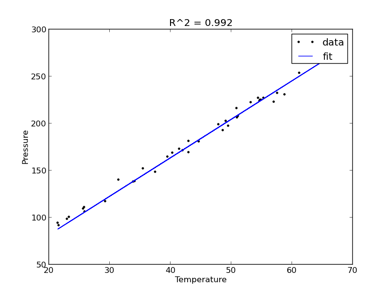
The fit is visually still pretty good, and the R^2 value is only slightly worse. Let us examine the residuals again.

residuals = P - np.dot(A,x)

plt.figure()
plt.plot(T,residuals,'ko')
plt.xlabel('Temperature')
plt.ylabel('residuals')
plt.savefig('images/model-selection-no-incpt-resid.png')

>>> <matplotlib.figure.Figure object at 0x0000000008A0F5C0>
[<matplotlib.lines.Line2D object at 0x000000000B29B0F0>]
<matplotlib.text.Text object at 0x000000000B276FD0>
<matplotlib.text.Text object at 0x000000000B283780>

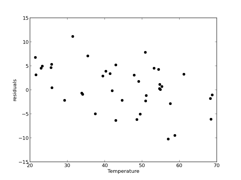
You can see a slight trend of decreasing value of the residuals as the Temperature increases. This may indicate a deficiency in the model with no intercept. For the ideal gas law in degC: \(PV = nR(T+273)\) or \(P = nR/V*T + 273*nR/V\), so the intercept is expected to be non-zero in this case. Specifically, we expect the intercept to be 273*R*n/V. Since the molar density of a gas is pretty small, the intercept may be close to, but not equal to zero. That is why the fit still looks ok, but is not as good as letting the intercept be a fitting parameter. That is an example of the deficiency in our model.

In the end, it is hard to justify a model more complex than a line in this case.

Copyright (C) 2013 by John Kitchin. See the License for information about copying.

org-mode source