Graphical methods to help get initial guesses for multivariate nonlinear regression

Posted February 18, 2013 at 09:00 AM | categories: data analysis, plotting | tags:

Updated February 27, 2013 at 02:40 PM

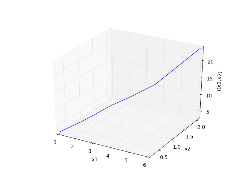
Fit the model f(x1,x2; a,b) = a*x1 + x2^b to the data given below. This model has two independent variables, and two parameters.

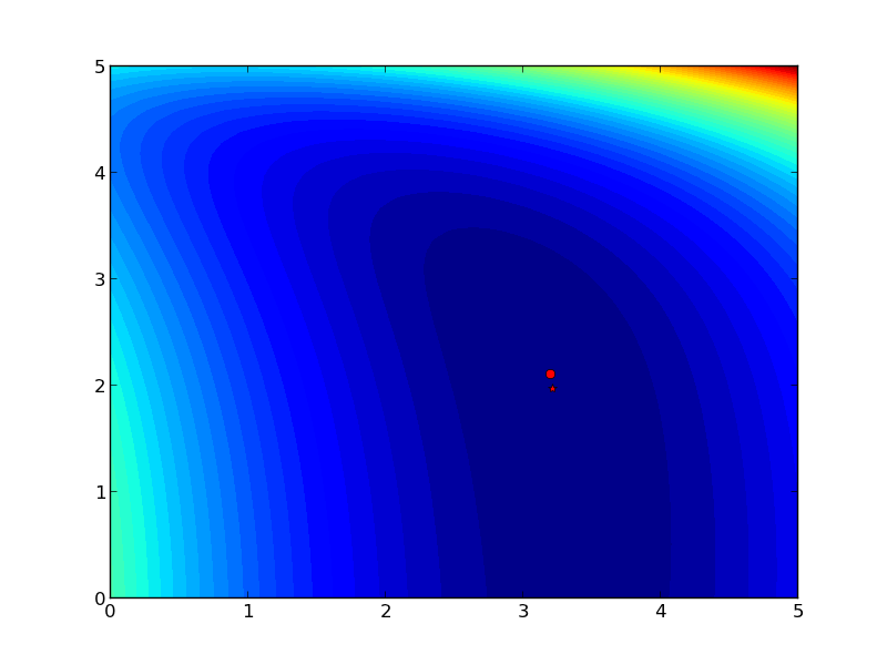
We want to do a nonlinear fit to find a and b that minimize the summed squared errors between the model predictions and the data. With only two variables, we can graph how the summed squared error varies with the parameters, which may help us get initial guesses. Let us assume the parameters lie in a range, here we choose 0 to 5. In other problems you would adjust this as needed.

import numpy as np
from mpl_toolkits.mplot3d import Axes3D
import matplotlib.pyplot as plt

x1 = [1.0, 2.0, 3.0, 4.0, 5.0, 6.0]
x2 = [0.2, 0.4, 0.8, 0.9, 1.1, 2.1]
X = np.column_stack([x1, x2]) # independent variables

f = [ 3.3079,    6.6358,   10.3143,   13.6492,   17.2755,   23.6271]

fig = plt.figure()
ax = fig.gca(projection = '3d')

ax.plot(x1, x2, f)
ax.set_xlabel('x1')
ax.set_ylabel('x2')
ax.set_zlabel('f(x1,x2)')

plt.savefig('images/graphical-mulvar-1.png')


arange = np.linspace(0,5);
brange = np.linspace(0,5);

A,B = np.meshgrid(arange, brange)

def model(X, a, b):
    'Nested function for the model'
    x1 = X[:, 0]
    x2 = X[:, 1]
    
    f = a * x1 + x2**b
    return f

@np.vectorize
def errfunc(a, b):
    # function for the summed squared error
    fit = model(X, a, b)
    sse = np.sum((fit - f)**2)
    return sse

SSE = errfunc(A, B)

plt.clf()
plt.contourf(A, B, SSE, 50)
plt.plot([3.2], [2.1], 'ro')
plt.figtext( 3.4, 2.2, 'Minimum near here', color='r')

plt.savefig('images/graphical-mulvar-2.png')

guesses = [3.18, 2.02]

from scipy.optimize import curve_fit

popt, pcov = curve_fit(model, X, f, guesses)
print popt

plt.plot([popt[0]], [popt[1]], 'r*')
plt.savefig('images/graphical-mulvar-3.png')

print model(X, *popt)

fig = plt.figure()
ax = fig.gca(projection = '3d')

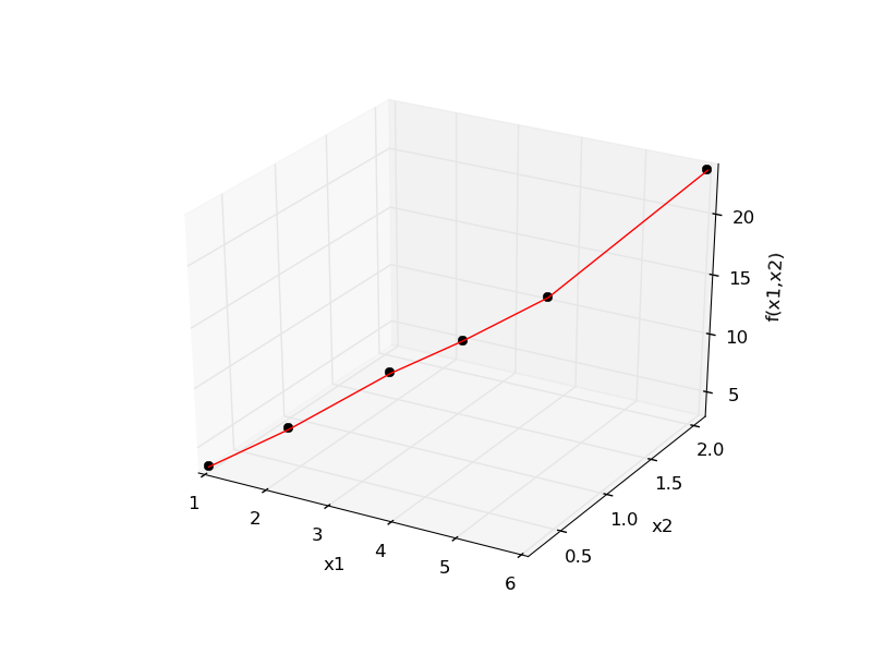
ax.plot(x1, x2, f, 'ko', label='data')
ax.plot(x1, x2, model(X, *popt), 'r-', label='fit')
ax.set_xlabel('x1')
ax.set_ylabel('x2')
ax.set_zlabel('f(x1,x2)')

plt.savefig('images/graphical-mulvar-4.png')

[ 3.21694798  1.9728254 ]
[  3.25873623   6.59792994  10.29473657  13.68011436  17.29161001
  23.62366445]

It can be difficult to figure out initial guesses for nonlinear fitting problems. For one and two dimensional systems, graphical techniques may be useful to visualize how the summed squared error between the model and data depends on the parameters.

org-mode source

The Kitchin Research Group

Chemical Engineering at Carnegie Mellon University

Graphical methods to help get initial guesses for multivariate nonlinear regression