Plane Poiseuille flow - BVP solve by shooting method
Posted February 15, 2013 at 09:00 AM | categories: bvp | tags: fluids
Updated March 08, 2013 at 10:08 AM
One approach to solving BVPs is to use the shooting method. The reason we cannot use an initial value solver for a BVP is that there is not enough information at the initial value to start. In the shooting method, we take the function value at the initial point, and guess what the function derivatives are so that we can do an integration. If our guess was good, then the solution will go through the known second boundary point. If not, we guess again, until we get the answer we need. In this example we repeat the pressure driven flow example, but illustrate the shooting method.
In the pressure driven flow of a fluid with viscosity \(\mu\) between two stationary plates separated by distance \(d\) and driven by a pressure drop \(\Delta P/\Delta x\), the governing equations on the velocity \(u\) of the fluid are (assuming flow in the x-direction with the velocity varying only in the y-direction):
$$\frac{\Delta P}{\Delta x} = \mu \frac{d^2u}{dy^2}$$
with boundary conditions \(u(y=0) = 0\) and \(u(y=d) = 0\), i.e. the no-slip condition at the edges of the plate.
we convert this second order BVP to a system of ODEs by letting \(u_1 = u\), \(u_2 = u_1'\) and then \(u_2' = u_1''\). This leads to:
\(\frac{d u_1}{dy} = u_2\)
\(\frac{d u_2}{dy} = \frac{1}{\mu}\frac{\Delta P}{\Delta x}\)
with boundary conditions \(u_1(y=0) = 0\) and \(u_1(y=d) = 0\).
for this problem we let the plate separation be d=0.1, the viscosity \(\mu = 1\), and \(\frac{\Delta P}{\Delta x} = -100\).
1 First guess
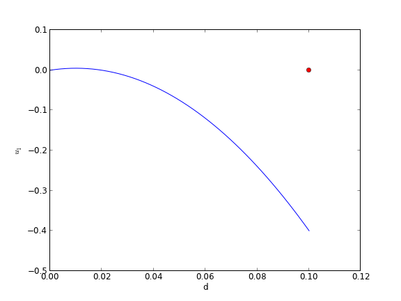
We need u_1(0) and u_2(0), but we only have u_1(0). We need to guess a value for u_2(0) and see if the solution goes through the u_2(d)=0 boundary value.
import numpy as np
from scipy.integrate import odeint
import matplotlib.pyplot as plt

d = 0.1 # plate thickness

def odefun(U, y):
    u1, u2 = U
    mu = 1
    Pdrop = -100
    du1dy = u2
    du2dy = 1.0 / mu * Pdrop
    return [du1dy, du2dy]

u1_0 = 0 # known
u2_0 = 1 # guessed

dspan = np.linspace(0, d)

U = odeint(odefun, [u1_0, u2_0], dspan)

plt.plot(dspan, U[:,0])
plt.plot([d],[0], 'ro')
plt.xlabel('d')
plt.ylabel('$u_1$')
plt.savefig('images/bvp-shooting-1.png')

Here we have undershot the boundary condition. Let us try a larger guess.
2 Second guess
import numpy as np
from scipy.integrate import odeint
import matplotlib.pyplot as plt

d = 0.1 # plate thickness

def odefun(U, y):
    u1, u2 = U
    mu = 1
    Pdrop = -100
    du1dy = u2
    du2dy = 1.0 / mu * Pdrop
    return [du1dy, du2dy]

u1_0 = 0 # known
u2_0 = 10 # guessed

dspan = np.linspace(0, d)

U = odeint(odefun, [u1_0, u2_0], dspan)

plt.plot(dspan, U[:,0])
plt.plot([d],[0], 'ro')
plt.xlabel('d')
plt.ylabel('$u_1$')
plt.savefig('images/bvp-shooting-2.png')

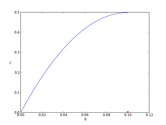
Now we have clearly overshot. Let us now make a function that will iterate for us to find the right value.
3 Let fsolve do the work
import numpy as np
from scipy.integrate import odeint
from scipy.optimize import fsolve
import matplotlib.pyplot as plt

d = 0.1 # plate thickness
Pdrop = -100
mu = 1

def odefun(U, y):
    u1, u2 = U
    du1dy = u2
    du2dy = 1.0 / mu * Pdrop
    return [du1dy, du2dy]

u1_0 = 0 # known
dspan = np.linspace(0, d)

def objective(u2_0):
    dspan = np.linspace(0, d)
    U = odeint(odefun, [u1_0, u2_0], dspan)
    u1 = U[:,0]
    return u1[-1]

u2_0, = fsolve(objective, 1.0)

# now solve with optimal u2_0
U = odeint(odefun, [u1_0, u2_0], dspan)

plt.plot(dspan, U[:,0], label='Numerical solution')
plt.plot([d],[0], 'ro')

# plot an analytical solution
u = -(Pdrop) * d**2 / 2 / mu * (dspan / d - (dspan / d)**2)
plt.plot(dspan, u, 'r--', label='Analytical solution')


plt.xlabel('d')
plt.ylabel('$u_1$')
plt.legend(loc='best')
plt.savefig('images/bvp-shooting-3.png')

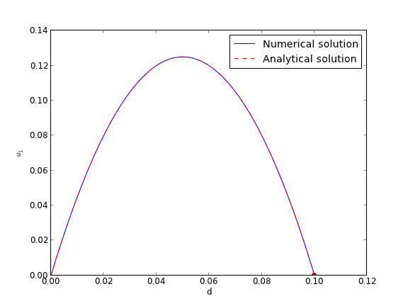
You can see the agreement is excellent!
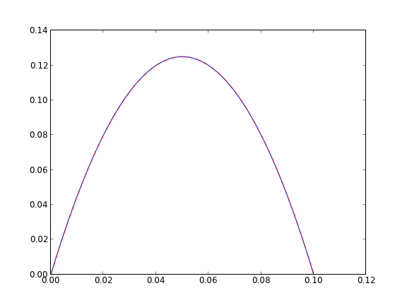
This also seems like a useful bit of code to not have to reinvent regularly, so it has been added to pycse as BVP_sh. Here is an example usage.
from pycse import BVP_sh
import matplotlib.pyplot as plt

d = 0.1 # plate thickness
Pdrop = -100
mu = 1

def odefun(U, y):
    u1, u2 = U
    du1dy = u2
    du2dy = 1.0 / mu * Pdrop
    return [du1dy, du2dy]

x1 = 0.0; alpha = 0.0
x2 = 0.1; beta = 0.0
init = 2.0 # initial guess of slope at x=0

X,Y = BVP_sh(odefun, x1, x2, alpha, beta, init)
plt.plot(X, Y[:,0])
plt.ylim([0, 0.14])

# plot an analytical solution
u = -(Pdrop) * d**2 / 2 / mu * (X / d - (X / d)**2)
plt.plot(X, u, 'r--', label='Analytical solution')
plt.savefig('images/bvp-shooting-4.png')
plt.show()

Copyright (C) 2013 by John Kitchin. See the License for information about copying.