The Kitchin Research Group

original post

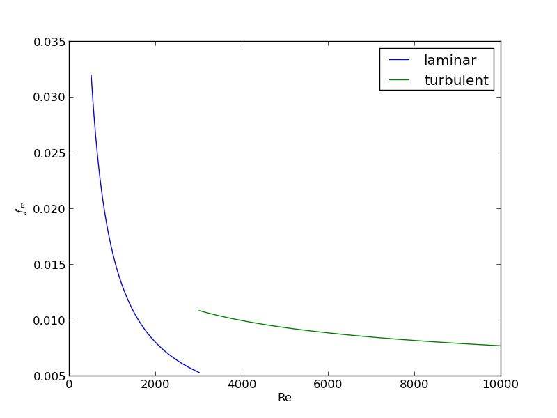
In Post 1280 we used a correlation for the Fanning friction factor for turbulent flow in a pipe. For laminar flow (Re < 3000), there is another correlation that is commonly used: \(f_F = 16/Re\). Unfortunately, the correlations for laminar flow and turbulent flow have different values at the transition that should occur at Re = 3000. This discontinuity can cause a lot of problems for numerical solvers that rely on derivatives.

Today we examine a strategy for smoothly joining these two functions. First we define the two functions.

import numpy as np
from scipy.optimize import fsolve
import matplotlib.pyplot as plt

def fF_laminar(Re):
    return 16.0 / Re

def fF_turbulent_unvectorized(Re):
    # Nikuradse correlation for turbulent flow
    # 1/np.sqrt(f) = (4.0*np.log10(Re*np.sqrt(f))-0.4)
    # we have to solve this equation to get f
    def func(f):
        return 1/np.sqrt(f) - (4.0*np.log10(Re*np.sqrt(f))-0.4)
    fguess = 0.01
    f, = fsolve(func, fguess)
    return f

# this enables us to pass vectors to the function and get vectors as
# solutions
fF_turbulent = np.vectorize(fF_turbulent_unvectorized)

Now we plot the correlations.

Re1 = np.linspace(500, 3000)
f1 = fF_laminar(Re1)

Re2 = np.linspace(3000, 10000)
f2 = fF_turbulent(Re2)

plt.figure(1); plt.clf()
plt.plot(Re1, f1, label='laminar')
plt.plot(Re2, f2, label='turbulent')
plt.xlabel('Re')
plt.ylabel('$f_F$')
plt.legend()
plt.savefig('images/smooth-transitions-1.png')

>>> >>> >>> >>> >>> <matplotlib.figure.Figure object at 0x051FF630>
[<matplotlib.lines.Line2D object at 0x05963C10>]
[<matplotlib.lines.Line2D object at 0x0576DD70>]
<matplotlib.text.Text object at 0x0577CFF0>
<matplotlib.text.Text object at 0x05798790>
<matplotlib.legend.Legend object at 0x05798030>

You can see the discontinuity at Re = 3000. What we need is a method to join these two functions smoothly. We can do that with a sigmoid function. Sigmoid functions

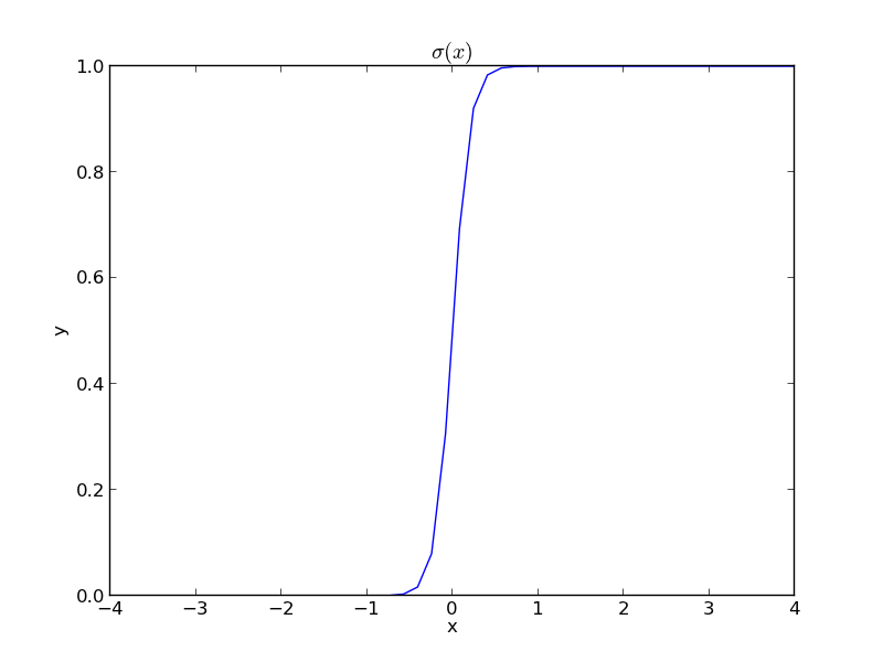
A sigmoid function smoothly varies from 0 to 1 according to the equation: \(\sigma(x) = \frac{1}{1 + e^{-(x-x0)/\alpha}}\). The transition is centered on \(x0\), and \(\alpha\) determines the width of the transition.

x = np.linspace(-4,4);
y = 1.0 / (1 + np.exp(-x / 0.1))
plt.figure(2); plt.clf()
plt.plot(x, y)
plt.xlabel('x'); plt.ylabel('y'); plt.title('$\sigma(x)$')
plt.savefig('images/smooth-transitions-sigma.png')

>>> <matplotlib.figure.Figure object at 0x0596CF10>
[<matplotlib.lines.Line2D object at 0x05A26D90>]
<matplotlib.text.Text object at 0x059A6050>
<matplotlib.text.Text object at 0x059AF0D0>
<matplotlib.text.Text object at 0x059BEA30>

If we have two functions, \(f_1(x)\) and \(f_2(x)\) we want to smoothly join, we do it like this: \(f(x) = (1-\sigma(x))f_1(x) + \sigma(x)f_2(x)\). There is no formal justification for this form of joining, it is simply a mathematical convenience to get a numerically smooth function. Other functions besides the sigmoid function could also be used, as long as they smoothly transition from 0 to 1, or from 1 to zero.

def fanning_friction_factor(Re):
    '''combined, continuous correlation for the fanning friction factor.
    the alpha parameter is chosen to provide the desired smoothness.
    The transition region is about +- 4*alpha. The value 450 was
    selected to reasonably match the shape of the correlation
    function provided by Morrison (see last section of this file)'''
    sigma =  1. / (1 + np.exp(-(Re - 3000.0) / 450.0));
    f = (1-sigma) * fF_laminar(Re) + sigma * fF_turbulent(Re)
    return f

Re = np.linspace(500,10000);
f = fanning_friction_factor(Re);

# add data to figure 1
plt.figure(1)
plt.plot(Re,f, label='smooth transition')
plt.xlabel('Re')
plt.ylabel('$f_F$')
plt.legend()
plt.savefig('images/smooth-transitions-3.png')

... ... ... ... ... ... ... ... >>> >>> >>> >>> ... <matplotlib.figure.Figure object at 0x051FF630>
[<matplotlib.lines.Line2D object at 0x05786310>]
<matplotlib.text.Text object at 0x0577CFF0>
<matplotlib.text.Text object at 0x05798790>
<matplotlib.legend.Legend object at 0x05A302B0>

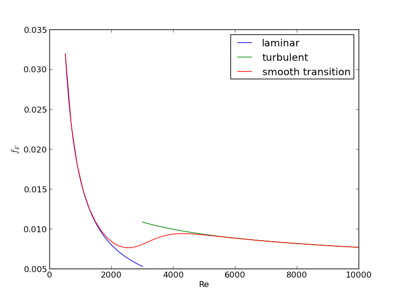
You can see that away from the transition the combined function is practically equivalent to the original two functions. That is because away from the transition the sigmoid function is 0 or 1. Near Re = 3000 is a smooth transition from one curve to the other curve.

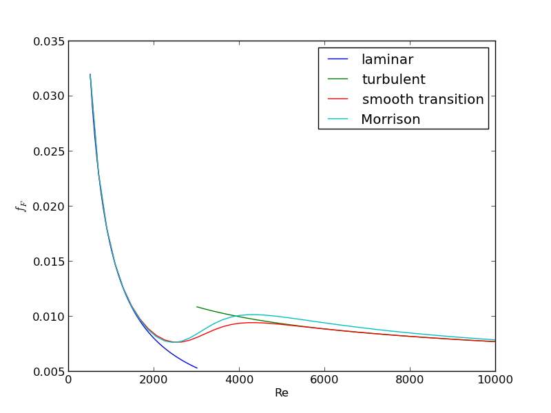
Morrison derived a single function for the friction factor correlation over all Re: \(f = \frac{0.0076\left(\frac{3170}{Re}\right)^{0.165}}{1 + \left(\frac{3171}{Re}\right)^{7.0}} + \frac{16}{Re}\). Here we show the comparison with the approach used above. The friction factor differs slightly at high Re, because Morrison's is based on the Prandlt correlation, while the work here is based on the Nikuradse correlation. They are similar, but not the same.

# add this correlation to figure 1
h, = plt.plot(Re, 16.0/Re + (0.0076 * (3170 / Re)**0.165) / (1 + (3170.0 / Re)**7))

ax = plt.gca()
handles, labels = ax.get_legend_handles_labels()

handles.append(h)
labels.append('Morrison')
ax.legend(handles, labels)
plt.savefig('images/smooth-transitions-morrison.png')

>>> >>> >>> >>> >>> >>> >>> <matplotlib.legend.Legend object at 0x05A5AEB0>

Copyright (C) 2013 by John Kitchin. See the License for information about copying.

org-mode source