The Kitchin Research Group

Matlab post

We often need to estimate parameters from nonlinear regression of data. We should also consider how good the parameters are, and one way to do that is to consider the confidence interval. A confidence interval tells us a range that we are confident the true parameter lies in.

In this example we use a nonlinear curve-fitting function: scipy.optimize.curve_fit to give us the parameters in a function that we define which best fit the data. The scipy.optimize.curve_fit function also gives us the covariance matrix which we can use to estimate the standard error of each parameter. Finally, we modify the standard error by a student-t value which accounts for the additional uncertainty in our estimates due to the small number of data points we are fitting to.

We will fit the function \(y = a x / (b + x)\) to some data, and compute the 95% confidence intervals on the parameters.

# Nonlinear curve fit with confidence interval
import numpy as np
from scipy.optimize import curve_fit
from scipy.stats.distributions import  t

x = np.array([0.5, 0.387, 0.24, 0.136, 0.04, 0.011])
y = np.array([1.255, 1.25, 1.189, 1.124, 0.783, 0.402])

# this is the function we want to fit to our data
def func(x, a, b):
    'nonlinear function in a and b to fit to data'
    return a * x / (b + x)

initial_guess = [1.2, 0.03]
pars, pcov = curve_fit(func, x, y, p0=initial_guess)

alpha = 0.05 # 95% confidence interval = 100*(1-alpha)

n = len(y)    # number of data points
p = len(pars) # number of parameters

dof = max(0, n - p) # number of degrees of freedom

# student-t value for the dof and confidence level
tval = t.ppf(1.0-alpha/2., dof) 

for i, p,var in zip(range(n), pars, np.diag(pcov)):
    sigma = var**0.5
    print 'p{0}: {1} [{2}  {3}]'.format(i, p,
                                  p - sigma*tval,
                                  p + sigma*tval)

import matplotlib.pyplot as plt
plt.plot(x,y,'bo ')
xfit = np.linspace(0,1)
yfit = func(xfit, pars[0], pars[1])
plt.plot(xfit,yfit,'b-')
plt.legend(['data','fit'],loc='best')
plt.savefig('images/nonlin-curve-fit-ci.png')

p0: 1.32753141454 [1.3005365922  1.35452623688]
p1: 0.0264615569701 [0.0236076538292  0.0293154601109]
(array([ 1.32753141,  0.02646156]), [[1.3005365921998688, 1.3545262368760884], [0.023607653829234403, 0.029315460110926929]], [0.0097228006732683319, 0.0010278982773703883])

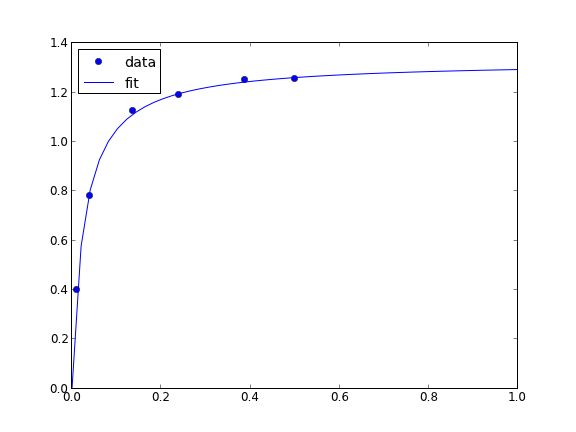
You can see by inspection that the fit looks pretty reasonable. The parameter confidence intervals are not too big, so we can be pretty confident of their values.

Copyright (C) 2013 by John Kitchin. See the License for information about copying.

org-mode source