
Introduction to 06-623, 06-713 and Jupyter Lab#
You are looking at a Jupyter notebook. This is an interactive computational environment that runs in your browser. We will use it all semester for lectures and assignments. This document is just a high level introduction to what they can do.
Jupyter notebooks are an interactive, browser-based tool for running Python. We will use them exclusively in this class.
We will use JupyterHUB exclusively this semester because it does not require any software installation or special hardware. You just need a browser and internet connection.
We will quickly build up the skills required to solve engineering problems. We will not learn everything about programming, mathematical modeling or engineering processes. My goal is to get you thinking about a very general computational way of thinking about these problems, and to learn how to use computation as a way to augment your analytical skills.
I will lecture from the notebooks, and show you how I use them. The notes will be available to you during class for you to work along with me.
The next cell is a code cell, and it can be exectued.
print("Hello World! Welcome to 06-623. We are going to have a lot fun!")
print(4)
a = 5  # variable assignment
print(a)
# Click the run button or
# C-Enter to run this cell
# Type shift-Enter to run this cell and go to the next one or create a new one.
# Lines that start with # are considered comments in Python
# Alt-Enter will run and insert a new cell
Hello World! Welcome to 06-623. We are going to have a lot fun!
4
5
This is a text cell. It is not executable, but is for people to read. You can embed narrative text, images, equations, etc in them.
Let’s describe a simple equation that we seek to solve. What is the value of \(a\) that satisfies the equation \(a + 4 = 5\)?
We can document our solution here, e.g. we find \(x\) by algebra. If we subtract 4 from each side of the equation, \(a\) will be isolated, and equal to the value of the right hand side of the equation.
Here is the code that implements that explanation:
a = 5 - 4
a  # this makes the value of x get displayed when it is the last line
1
# alternatively, you can print it explicitly
print(a)
1
print(5 - 4)
1
numpy#
numpy is a Python library for arrays. We have to import this library to access the functionality in it. The conventional way to import this library is:
import numpy as np
To see help on the numpy library, run this cell:
?np
Now, we can access functions in the numpy module using “dot notation”. For example, let us start by creating an array of linearly spaced points using the linspace function. First, we access the help to see how to use it.
?np.linspace
np.pi
3.141592653589793
x = np.linspace(0, 2 * np.pi)
x
array([0.        , 0.12822827, 0.25645654, 0.38468481, 0.51291309,
       0.64114136, 0.76936963, 0.8975979 , 1.02582617, 1.15405444,
       1.28228272, 1.41051099, 1.53873926, 1.66696753, 1.7951958 ,
       1.92342407, 2.05165235, 2.17988062, 2.30810889, 2.43633716,
       2.56456543, 2.6927937 , 2.82102197, 2.94925025, 3.07747852,
       3.20570679, 3.33393506, 3.46216333, 3.5903916 , 3.71861988,
       3.84684815, 3.97507642, 4.10330469, 4.23153296, 4.35976123,
       4.48798951, 4.61621778, 4.74444605, 4.87267432, 5.00090259,
       5.12913086, 5.25735913, 5.38558741, 5.51381568, 5.64204395,
       5.77027222, 5.89850049, 6.02672876, 6.15495704, 6.28318531])
Most mathematical operations are element-wise on arrays.
x - x
array([0., 0., 0., 0., 0., 0., 0., 0., 0., 0., 0., 0., 0., 0., 0., 0., 0.,
       0., 0., 0., 0., 0., 0., 0., 0., 0., 0., 0., 0., 0., 0., 0., 0., 0.,
       0., 0., 0., 0., 0., 0., 0., 0., 0., 0., 0., 0., 0., 0., 0., 0.])
x * x
array([0.00000000e+00, 1.64424896e-02, 6.57699585e-02, 1.47982407e-01,
       2.63079834e-01, 4.11062241e-01, 5.91929627e-01, 8.05681992e-01,
       1.05231934e+00, 1.33184166e+00, 1.64424896e+00, 1.98954125e+00,
       2.36771851e+00, 2.77878075e+00, 3.22272797e+00, 3.69956017e+00,
       4.20927735e+00, 4.75187950e+00, 5.32736664e+00, 5.93573876e+00,
       6.57699585e+00, 7.25113793e+00, 7.95816498e+00, 8.69807701e+00,
       9.47087403e+00, 1.02765560e+01, 1.11151230e+01, 1.19865749e+01,
       1.28909119e+01, 1.38281338e+01, 1.47982407e+01, 1.58012325e+01,
       1.68371094e+01, 1.79058712e+01, 1.90075180e+01, 2.01420498e+01,
       2.13094666e+01, 2.25097683e+01, 2.37429550e+01, 2.50090267e+01,
       2.63079834e+01, 2.76398251e+01, 2.90045517e+01, 3.04021633e+01,
       3.18326599e+01, 3.32960415e+01, 3.47923081e+01, 3.63214596e+01,
       3.78834961e+01, 3.94784176e+01])
x @ x # dot-product -> leads to a constant
np.float64(664.687643338671)
x**2
array([0.00000000e+00, 1.64424896e-02, 6.57699585e-02, 1.47982407e-01,
       2.63079834e-01, 4.11062241e-01, 5.91929627e-01, 8.05681992e-01,
       1.05231934e+00, 1.33184166e+00, 1.64424896e+00, 1.98954125e+00,
       2.36771851e+00, 2.77878075e+00, 3.22272797e+00, 3.69956017e+00,
       4.20927735e+00, 4.75187950e+00, 5.32736664e+00, 5.93573876e+00,
       6.57699585e+00, 7.25113793e+00, 7.95816498e+00, 8.69807701e+00,
       9.47087403e+00, 1.02765560e+01, 1.11151230e+01, 1.19865749e+01,
       1.28909119e+01, 1.38281338e+01, 1.47982407e+01, 1.58012325e+01,
       1.68371094e+01, 1.79058712e+01, 1.90075180e+01, 2.01420498e+01,
       2.13094666e+01, 2.25097683e+01, 2.37429550e+01, 2.50090267e+01,
       2.63079834e+01, 2.76398251e+01, 2.90045517e+01, 3.04021633e+01,
       3.18326599e+01, 3.32960415e+01, 3.47923081e+01, 3.63214596e+01,
       3.78834961e+01, 3.94784176e+01])
We can define new variables
y1 = np.sin(x)
y2 = np.cos(x)
y2
array([ 1.        ,  0.99179001,  0.96729486,  0.92691676,  0.8713187 ,
        0.80141362,  0.71834935,  0.6234898 ,  0.51839257,  0.40478334,
        0.28452759,  0.1595999 ,  0.03205158, -0.09602303, -0.22252093,
       -0.34536505, -0.46253829, -0.57211666, -0.67230089, -0.76144596,
       -0.8380881 , -0.90096887, -0.94905575, -0.98155916, -0.99794539,
       -0.99794539, -0.98155916, -0.94905575, -0.90096887, -0.8380881 ,
       -0.76144596, -0.67230089, -0.57211666, -0.46253829, -0.34536505,
       -0.22252093, -0.09602303,  0.03205158,  0.1595999 ,  0.28452759,
        0.40478334,  0.51839257,  0.6234898 ,  0.71834935,  0.80141362,
        0.8713187 ,  0.92691676,  0.96729486,  0.99179001,  1.        ])
plotting#
We can make plots using matplotlib. This cell imports the plotting library. These should be used in this order.
import matplotlib.pyplot as plt
You call functions in the plt library to create plots. These are automatically saved in the notebook.
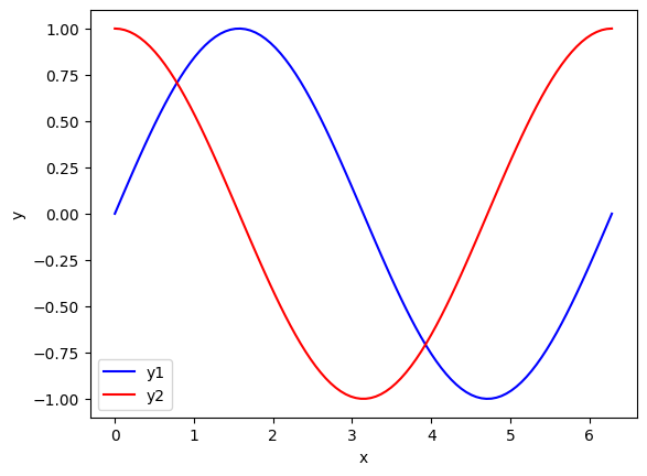
x = np.linspace(0, 2 * np.pi, 100)
y1 = np.sin(x)
y2 = np.cos(x)
plt.plot(x, y1, "b-", x, y2, "r-")
plt.xlabel("x")
plt.ylabel("y")
plt.legend(["y1", "y2"])
# Always include axis labels and legends when appropriate
<matplotlib.legend.Legend at 0x7fde41b104d0>
scipy#
scipy contains numerous libraries for a broad range of scientific computing needs.
Suppose we want to perform the following integral: \(I = \int_0^{4.5} J_{2.5}(x) dx\). The function \(J_{2.5}\) is a special function known as a Bessel function. scipy provides both the integration function, and an implementation of the special function we can use.
This is not code you need to memorize now; it is an example of the kind of code we will learn to write.
from scipy.integrate import quad
from scipy.special import jv
?quad
?jv
To evaluate this integral, we have to define a function for the integrand, and use the quad function to compute the integral. The quad function returns two values, the value of the integral, and an estimate of the maximum error in the integral.
# This is how we define a function. There is a function name, and arguments
# The function returns the output of the jv function.
def integrand(x):
    return jv(2.5, x)


I, err = quad(integrand, 0, 4.5)

I, err
(1.1178179380783253, 7.866317216380692e-09)
Summary#
Today we introduced several ideas about using Jupyter notebooks to run Python computations. The main points are:
Code is run in code cells
You have to import some functions from libraries
numpy, scipy and matplotlib are three of the main scientific programming libraries we will use a lot.
We saw some ways to get help on functions
Next time we will dig into defining functions more deeply, and how to print formatted strings containing results.
Getting a PDF from a Jupyter notebook#
The first thing you have to do is open a Terminal. This will trigger the installation of Chromium, which is used to convert HTML to PDF. You only have to do this once.
Go to the File->Save and Export Notebook As->Webpdf
A PDF file should automatically be created and download in your browser in a new tab. Note you can also use PDF instead; this uses LaTeX to create a PDF. It may be nicer looking, but it is more fragile and does not always work.
Additional resources#
Check out the pycse playlist on YouTube.
See Point Breeze Publications, LLC for a series of booklets on pycse on different topics (some are advanced).
Explore the Help menu in Jupyter Lab.
Some review material#
Below you will find a quiz, and some flash cards. When you run the cells, you will get an interactive widget you can use to test your understanding. The results are not persistent, and they will disappear when you close the notebook.
from jupyterquiz import display_quiz
display_quiz('.quiz.json')
Run this cell. Click on the card to see the other side. Click Next to see the next card.
from jupytercards import display_flashcards
display_flashcards('flash.json')