Path Following & Inverse Mapping
Tracing how a solution moves as a parameter changes is a re-solve loop by default: pick the next \(\theta\), solve the NLP, repeat. POUNCE replaces most of those solves with a back-solve on the KKT factor it already holds. Given the converged factor at one point, the sensitivity \(\partial x^*/\partial\theta\) is available for the cost of a triangular solve, so a step along the path is a prediction rather than an optimization.
PathFollower (in both pounce.jax and pounce.torch) wraps that idea
in a predictor–corrector loop:
- predict — extrapolate \(x\) and the multipliers along the
held-factor sensitivity (
jvp_from_state); - monitor — without solving, check the KKT residual at the predicted point and the active-set margin;
- correct — only when the monitor trips, take one warm-started,
barrier-\(\mu\) seeded re-solve that also re-anchors the factor
(
warm_anchor).
On a linear-response problem the predictor is exact and a whole path costs one solve. On a curved problem the monitor tolerance is the lever: loosen it to accept more predictor steps between re-solves.
The parametric problem
Everything on this page traces the solution of
\[ \min_x; f(x, \theta) \quad \text{s.t.} \quad g(x, \theta) = 0,; \mathrm{lb} \le x \le \mathrm{ub} \]
as \(\theta\) varies. Build it as a JaxProblem (or TorchProblem —
the API is identical, see Python API):
import jax.numpy as jnp
from pounce.jax import JaxProblem, PathFollower

def f(x, p):
    return jnp.sum((x - p) ** 2)

def g(x, p):
    return jnp.stack([x[0] + x[1] - 1.0])

jp = JaxProblem(
    f=f, g=g, n=2, m=1, p_example=jnp.zeros(2),
    lb=jnp.full(2, -5.0), ub=jnp.full(2, 5.0),
    cl=jnp.zeros(1), cu=jnp.zeros(1),
    options={"tol": 1e-9, "print_level": 0, "sb": "yes"},
)
Parameter continuation: follow
follow traces \(x^*(\theta(s))\) for a prescribed path
\(\theta(s)\), \(s \in [s_0, s_1]\). This is the operability-tracing
and uncertainty-mapping case: \(s\) is monotone by construction, so the
path cannot fold in \(s\).
def circle(s):
    a = 2.0 * jnp.pi * s
    return jnp.array([0.5 + 0.4 * jnp.cos(a), 0.4 * jnp.sin(a)])

pf = PathFollower(jp, monitor_tol=1e-6, ds0=0.05)
tr = pf.follow(circle, (0.0, 1.0), jnp.zeros(2))

print(tr.n_steps, tr.n_correctors, tr.n_accepts)
# 7 0 7   -> one anchor solve for the whole loop; naive would be 8
The objective here is quadratic, so \(\partial x^*/\partial\theta\) is constant, the predictor is exact, and the monitor never fires: zero correctors. Add curvature and the trade-off appears. With
def f_nl(x, p):
    return jnp.sum((x - p) ** 2) + 0.02 * jnp.sum(x ** 4)
around the same loop (ds0=0.05, ds_max=0.1), sweeping monitor_tol
against the error versus a cold solve at every recorded \(\theta\):
monitor_tol | solves | accepts | max path error |
|---|---|---|---|
1e-6 | 10 | 2 | 9e-15 |
1e-3 | 9 | 3 | 2e-4 |
5e-3 | 5 | 7 | 9e-4 |
2e-2 | 3 | 9 | 2e-3 |
(12 solves if you re-solved at every step.) That is the whole predictor–corrector lever: you are paying accuracy for solves at a rate you set.
Result: PathTrace
Both entry points return a PathTrace dataclass:
| Field | Meaning |
|---|---|
s | path parameter at each recorded point (arclength in arclength mode) |
theta, x, lam | parameter, primal, and multipliers along the path |
n_steps | steps taken |
n_correctors | of those, how many needed a solve |
n_accepts | accepted on the predictor alone (no solve) |
active_set_changes | s values where the active set changed |
turning_points | \(\theta\) at detected folds (arclength mode) |
status | "ok", or a reason string on early stop |
n_correctors vs n_steps is the headline number: it is how many NLP
solves you avoided.
Step-size adaptation
The step grows by grow on an accepted predictor or an easy correction
(≤ 3 IPM iterations), shrinks by shrink on a hard one (≥ 10 iterations)
or a failed correction, and is clamped to [ds_min, ds_max]. When a
correction reveals the active set changed, the step resets to ds0
and the region is resolved finely — the s value is recorded in
active_set_changes. If a correction fails and the step would drop below
ds_min, the trace stops with status="corrector_failed" rather than
silently returning garbage.
The active_margin_tol knob is what keeps the predictor honest near a
critical-region boundary: a predicted point closer than this to an
active-set change forces a correction, so the predictor never
extrapolates across the discontinuity.
Tracing past folds: trace_arclength
Parameter continuation stalls at a turning point, where
\(\partial x^*/\partial\theta\) is singular and the path doubles back in
\(\theta\). trace_arclength parametrises the solution curve by
arclength instead, solving the stationarity/feasibility system
\[ R(x, \lambda, \theta) = \begin{bmatrix} \nabla_x f + J_g^{\mathsf T}\lambda \\ g \end{bmatrix} = 0 \]
along its curve in \((x, \lambda, \theta)\) space, with a tangent predictor and a Newton corrector on the augmented system \([R;\ \text{arclength}]\). Because arclength never reverses, the trace passes straight through the fold.
The classic test: the stationarity of \(f = x^4/4 - x^2/2 - \theta x\) is \(\theta = x^3 - x\), which folds at \(x = \pm 1/\sqrt3\) (\(\theta = \mp 0.385\)).
def f_cubic(x, p):
    th = p[0]
    return x[0] ** 4 / 4.0 - x[0] ** 2 / 2.0 - th * x[0]

jp_c = JaxProblem(f=f_cubic, g=None, n=1, m=0, p_example=jnp.zeros(1),
                  options={"tol": 1e-10, "print_level": 0, "sb": "yes"})

trc = PathFollower(jp_c).trace_arclength(
    jnp.array([-1.3]), -0.4, ds=0.05, n_steps=120,
)
print(trc.turning_points)   # [0.3843, -0.3805]
Both folds are found, in the order the trace reaches them, to the
accuracy of the ds=0.05 sampling — the exact values are
\(\pm 2/(3\sqrt3) = \pm 0.3849\). They are recorded where the
\(\theta\)-component of the tangent changes sign, so tighten ds if
you need the turning point located more precisely.
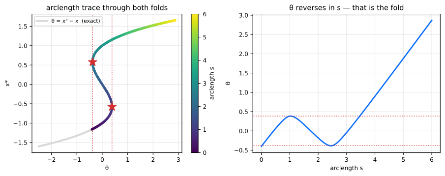
Colour is arclength, so the trace reads as one continuous walk: up the lower branch, through the first fold (star), back across the middle branch, through the second fold, and out along the upper branch. The right panel is the same run against arclength — \(\theta\) rises, reverses, and rises again. Those reversals are precisely where a method that treats \(\theta\) as the independent variable has nowhere to go.
(Regenerate with python3 scripts/make-docs-figures.py.)
direction sets the sign of the initial step in \(\theta\);
newton_tol / newton_max control the corrector.
Chemical-engineering example: phase envelopes and inverse design
The phase boundary of a multicomponent mixture is a natural fold problem. With equilibrium ratios \(K_i=y_i/x_i\), a fixed vapor fraction \(\beta\), and a Peng–Robinson fugacity model, an isopleth is the square system
\[ \log K_i + \log\phi_i^v(y,T,P)-\log\phi_i^l(x,T,P)=0, \qquad \sum_i(y_i-x_i)=0. \]
A pressure ladder stops at the cricondenbar, while a prescribed-parameter predictor can silently land on the algebraically exact but physically vacuous \(K_i=1\) branch. Pseudo-arclength continuation passes the fold. For a quantitative extremum, the example then solves the augmented simple-fold system
\[ F(x,\theta,q)=0,\qquad F_xv=0,\qquad v^Tv=1, \]
where \(q\) contains \(N-1\) unconstrained log-ratio composition coordinates and one binary interaction parameter \(k_{ij}\). This removes the arclength-grid error from the reported cricondenbar or cricondentherm and makes the refined extremum differentiable with respect to the physical design.
Notebook
34_phase_envelope_peng_robinson.ipynb
contains the complete workflow and uses the tested
pounce.examples.phase_envelope implementation. It independently reproduces
the 282.53 K methane/propane maxcondentherm reported by
Deiters and Bell (2019), validates every
binary design derivative by central perturbations that each retrace the full
envelope, and verifies an inverse composition design with another fresh trace.
The guards in the example check equation residuals, composition normalization, distance from the trivial branch, and admissibility of the selected cubic roots. They are deliberately described as local guards: a production flash or envelope code should also perform a global tangent-plane-distance stability test and should not treat this example module as a general property package.
Inverse / uncertainty mapping: inverse_map_rhs
A related problem runs the map backwards: given a prescribed path in output space, what input path produces it? For an output \(y = h(x^*(\theta), \theta)\) of the embedded optimizer, the Alves–Kitchin–Lima inverse map integrates
\[ \frac{d\theta}{ds} = \Big(\frac{\partial y}{\partial \theta}\Big)^{-1} \frac{dy}{ds}, \qquad \frac{\partial y}{\partial \theta} = \frac{\partial h}{\partial x} J + \frac{\partial h}{\partial \theta}, \]
with \(J = \partial x^*/\partial\theta\) off the held factor and the output Jacobians by autodiff. Note this is a linear solve against the sensitivity, not a Jacobian-vector product, so \(\partial y/\partial \theta\) must be square: the output dimension must equal the parameter dimension (with the default identity output, \(n = p\)).
inverse_map_rhs builds the right-hand side and hands the stepping to an
off-the-shelf integrator — no hand-rolled stepper, no NLP inversion:
Here the output is the solution itself (\(h = x^*\), the default), and \(f = (x - \theta)^2 + 0.05x^4\) makes the map explicit (\(\theta = y + 0.1y^3\)) so the trace can be checked analytically:
import diffrax
from pounce.jax import inverse_map_rhs

def f_inv(x, p):
    return (x[0] - p[0]) ** 2 + 0.05 * x[0] ** 4

jp_inv = JaxProblem(f=f_inv, g=None, n=1, m=0, p_example=jnp.zeros(1),
                    options={"tol": 1e-11, "print_level": 0, "sb": "yes"})

# A closed loop in output space, and its velocity.
y_of_s = lambda s: jnp.array([0.5 + 0.3 * jnp.sin(2 * jnp.pi * s)])
dy_ds  = lambda s: jnp.array([0.3 * 2 * jnp.pi * jnp.cos(2 * jnp.pi * s)])

rhs = inverse_map_rhs(jp_inv, dy_ds)        # f(s, θ) -> dθ/ds
y0 = float(y_of_s(0.0)[0])
theta0 = jnp.array([y0 + 0.1 * y0 ** 3])    # θ0 with x*(θ0) = y(0)

term = diffrax.ODETerm(lambda s, theta, args: rhs(s, theta))
sol = diffrax.diffeqsolve(
    term, diffrax.Dopri5(), t0=0.0, t1=1.0, dt0=0.01, y0=theta0,
    stepsize_controller=diffrax.PIDController(rtol=1e-9, atol=1e-11),
    max_steps=100_000,
)
A closed loop in output space must come back to a closed loop in input space; that round trip is the cheapest correctness check you have on an inverse map.
Under JAX the whole evaluation (solve, sensitivity, output Jacobians,
linear solve) rides one jax.pure_callback, so the RHS is traceable and
composes under jax.jit and diffrax. Under PyTorch it is a plain
callable — drop it into scipy.integrate or torchdiffeq.
warm=True warm-starts each inner solve from the previous evaluation’s
primal, duals, and barrier \(\mu\). The converged \(x^*(\theta)\) is
unique, so the result is unchanged up to solver tolerance; only the
iteration count drops, by a measured ~1.4–1.7× on smooth low-dimensional
maps. Interior-point methods warm-start weakly, so if the NLP is
expensive and the map is smooth, prefer PathFollower — its predictor
skips solves entirely rather than making each one cheaper.
When to use which
| Situation | Use |
|---|---|
| Active set may change along the path | PathFollower.follow — the robust default |
| The path folds (singular \(\partial x^*/\partial\theta\)) | PathFollower.trace_arclength |
| Smooth map, fixed active set, want adaptive stepping / dense output | inverse_map_rhs + diffrax / scipy |
All three run on the same held KKT factor; a predict step is one back-solve, never an NLP re-solve.
Scope and limitations
PathFollower supports equality constraints (cl == cu) and
variable bounds. Two-sided inequalities (cl != cu) are rejected with an
explicit error rather than silently mis-traced: the smooth-drift
monitor’s constraint residual (max|g|, valid only at \(g = 0\)) and
the arclength system \(R\) (which treats every row as \(g = 0\)) are
not valid for them. Reformulate inequalities with slack equalities.
trace_arclength additionally requires a scalar parameter and a
fixed active set along the traced branch; use follow for a
multi-dimensional path. Bifurcation and branch switching, Hopf detection,
general DAE continuation, and inequality-active folds are out of scope.
See also
notebooks/14_path_following.ipynb— runnable tour of all of the above, with the analytic checks.examples/inverse_map_diffrax.py— standalone 2-D coupled inverse map with a round-trip check.- Sensitivity Analysis — the underlying \(\partial x^*/\partial\theta\) and the active-set margin.
- Python API —
JaxProblem/TorchProblem, anchoring, and factor lifetime.