Choosing a Solver
POUNCE is not a single solver but a small family of them sharing one numerical backbone. This page is the map: what each solver is, when to reach for it, and how they fit together.
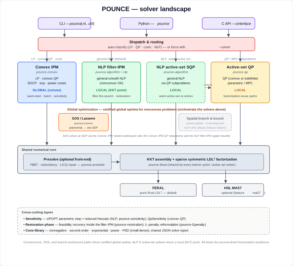
The one-sentence version: convex and conic problems are solved to the global
optimum; nonconvex problems are solved locally by default, or to a certified
global optimum via the SOS (polynomial) and spatial branch-and-bound (general)
paths. Every solver, whatever its flavor, ultimately factorizes a symmetric
KKT system through the shared pounce-linsol layer, which in turn drives a
pluggable backend (FERAL by default, HSL MA57 optionally).
The solvers at a glance
| Solver | Problem class | Optimum | Crate | Entry points |
|---|---|---|---|---|
| NLP filter-IPM | general smooth NLP (nonconvex OK) | local (KKT) | pounce-algorithm + pounce-nlp | CLI default; Python Problem/minimize; solver_selection=nlp |
| NLP active-set SQP | general smooth NLP | local | pounce-algorithm (subproblems via pounce-qp) | algorithm=active-set-sqp |
| Convex IPM (LP/QP) | LP, convex QP | global | pounce-convex | solve_qp_ipm; pounce.qp.solve_qp; solver_selection=lp-ipm/qp-ipm |
| Convex IPM (conic) | SOCP, exp/power/PSD cones, convex QCQP | global | pounce-convex | solve_socp_ipm; pounce.qp.solve_socp; minimize (convex QCQP); solver_selection=socp; pounce <file>.cbf |
| Active-set QP | QP (linear rows), convex or indefinite | local | pounce-qp | ParametricActiveSetSolver; pounce.qp.solve_qp(method="active-set"); solver_selection=qp-active-set — opt-in only; auto never picks it (see note) |
| SOS / Lasserre | polynomial (nonconvex) | global | pounce-convex | sos_minimize; pounce.sos_minimize |
When to reach for the active-set QP.
autonever selects it: a cold, one-shot convex QP goes to the interior-point path, which is materially more robust on that workload (137 of the 138 Maros-Mészáros problems, against substantially fewer for a cold active-set solve). That is the character of the method rather than a defect — an active-set iteration count is combinatorial in the size of the active set, while an interior-point count is nearly independent of problem size. Choosesolver_selection=qp-active-setwhen you want an exact vertex solution, or when you are solving a sequence of similar QPs — MPC steps, branch-and-bound nodes, continuation — where the working set carries across solves andsolve_parametriccan trace the homotopy from the previous solution instead of starting over.
POUNCE has no spatial branch-and-bound solver for general factorable nonconvex NLPs — no
solver_selection=globalCLI route, nominimize_globalPython entry point. The only certified-global path for a nonconvex problem is SOS / Lasserre, and it covers polynomials only.
When to choose each
General nonlinear program (the common case) → NLP filter-IPM
If your model has nonlinear objective or constraints and you don’t know (or can’t assume) convexity, this is the default and the most mature path. It is POUNCE’s port of Ipopt’s filter line-search interior-point method: robust on nonconvex problems, with a feasibility restoration phase for hard starts and exact or limited-memory Hessians. It returns a local KKT point — for a nonconvex problem there is no global guarantee.
- CLI:
pounce model.nl(or a built-in problem). - Python: the cyipopt-style
Problemclass, or the scipy-styleminimizefacade. - Reach for limited-memory Hessians (
hessian_approximation=limited-memory) when second derivatives are unavailable or expensive.
A sequence of related NLPs, or a stable active set → NLP active-set SQP
Selected with algorithm=active-set-sqp. It solves the NLP as a sequence
of quadratic subproblems (handed to pounce-qp), which warm-starts
extremely well when the active set is stable across solves — e.g. a
parametric sweep or a control loop. For a single cold solve of a general
NLP, prefer the filter-IPM.
Linear or convex quadratic program → Convex IPM (LP/QP)
If P ⪰ 0 (or P = 0 for an LP), use the convex interior-point solver:
it returns the global optimum, detects primal/dual infeasibility, and
offers warm-starting, batched and multiple-RHS solving, a build-once /
solve-many QpFactorization handle, and post-optimal sensitivity
(QpSensitivity — the sIPOPT analog). The CLI’s auto routing classifies
an .nl and sends LP/convex-QP problems here automatically, and a .nl
carrying the sIPOPT sens_* suffixes is now answered here rather than
rerouted to the general NLP engine — see
LP/QP routing
for what still routes away and why.
- Python:
pounce.qp.solve_qp(andsolve_qp_batch,solve_qp_multi_rhs).
Second-order, exponential, or power cones → Convex IPM (conic)
The same convex solver handles conic programs: second-order cones, the
exponential and power cones that express geometric programming,
entropy / log-sum-exp, logistic models, and p-norm constraints, and the
positive-semidefinite cone for small dense SDPs. Also global. This
is the path to use when you can cast a nominally-nonconvex problem into a
convex cone — you trade modeling effort for a global guarantee. (The PSD
cone is self-scaled and runs on the symmetric driver; the exp/power cones
run on the non-symmetric HSDE driver, so the two families can’t yet be
mixed in one problem.)
A common special case routes here automatically: a convex
quadratically-constrained QP (QCQP). When auto routing finds a
convex-quadratic inequality ½xᵀHx + aᵀx + b ≤ 0 (H ⪰ 0), it reformulates
each such constraint to one second-order cone (H = FᵀF) and sends the whole
problem to the conic solver — no .cbf and no manual cone bookkeeping needed.
This works from a .nl/Pyomo model on the CLI and from minimize() in Python
(which probes each constraint’s Hessian and only routes when it can prove the
feasible set is convex). See LP / QP Solver Routing.
- Python:
pounce.qp.solve_socp(..., cones=[("exp", 3), ("pow", 0.5), ...])for an explicit cone program, or justminimize(...)for a convex QCQP. - CLI: a Conic Benchmark Format file,
pounce model.cbf(see the CBLIB benchmark tier), or any convex-QCQP.nlunderautorouting.
Nonconvex problem, global optimum required → SOS (polynomials only)
When the problem is genuinely nonconvex and a local optimum is not good enough, the one path to a certified global optimum is for polynomials:
- Polynomial objective/constraints → SOS / Lasserre (
sos_minimize, orpounce.sos_minimize). A single semidefinite program certifies the global minimum (the largestγwithp − γin the Putinar cone), and the global minimizers are recovered from the moment matrix — even multiple ones, via a facial-reduction step. Best for modest degree and dimension; the SDP grows with the relaxation order.
If the problem is nonconvex and not polynomial (exp/ln/trig), POUNCE
cannot certify a global optimum. Reformulate into the convex cone library if
you can; otherwise multistart the local NLP solver and accept that the result
is uncertified.
See Global Optimization for the SOS path in depth, and for the multistart fallback.
Indefinite QP, or a QP inner-solver → Active-set QP
pounce-qp is a sparse parametric active-set solver that accepts an
indefinite Hessian (via inertia control), with two-sided bounds and
factorization-reuse across a homotopy. It is the engine behind the
active-set SQP path, and is the right choice for MPC-style problems or any
setting where you re-solve a slowly-changing QP many times. Use the convex
IPM instead when P ⪰ 0 and you want a single robust solve with
infeasibility certificates.
It is the only entry point here that will take an indefinite P; both the
convex IPM and the conic solver refuse one, because without a PSD Hessian the
IPM’s optimality test accepts a saddle point and reports it as optimal
(issue #112). Ask for the engine by name:
from pounce.qp import solve_qp
r = solve_qp(P=P_indefinite, c=c, lb=lb, ub=ub, method="active-set")
pounce model.nl solver_selection=qp-active-set # class: nonconvex QP
Two things to hold onto about the answer. It is local: a nonconvex QP can
have many KKT points, and what you get is the one the active set walked to,
the same guarantee minimize gives on a nonconvex NLP. It is at least a
minimum, though, which took a fix — inertia control leaves the first-order
conditions satisfied at a saddle, and until
issue #848 the engine
reported one as optimal (min ½xᵀ[[1,5],[5,1]]x over [−1,1]² came back at
objective 0 against a true minimum of −4). From 0.11.0 two guards stand behind an
optimal here. The engine tests the reduced Hessian on its working set’s null
space, and when it finds a feasible direction of negative curvature it follows
it — to a better point, to an unbounded verdict if nothing blocks it, or to
an honest non-optimal status if it runs out of budget. The driver then
screens the result by exhibition, refusing a verdict only where it can walk a
direction and hand you a strictly better feasible point; that one is not
confined to the working set’s null space, so it reaches negative curvature
hidden behind a bound whose multiplier is exactly zero, which the first cannot
see. What you do not get is a global minimum, or a guarantee in the case
where neither guard concludes — the first-order verdict stands there, as it
always did. And the constraints
must be linear — the curvature this engine controls is the objective’s, so
an indefinite objective over any quadratic row, convex row or not, is a
nonconvex QCQP and goes to the NLP filter-IPM instead (see
LP/QP routing).
How to override the automatic routing
The CLI classifies each .nl problem and picks a solver, but you can force
the choice:
pounce model.nl solver_selection=auto          # default: classify, then route
pounce model.nl solver_selection=nlp           # filter-IPM (or active-set-sqp via algorithm=)
pounce model.nl solver_selection=lp-ipm        # convex LP interior-point
pounce model.nl solver_selection=qp-ipm        # convex QP interior-point
pounce model.nl solver_selection=socp          # conic interior-point (convex QCQP)
pounce model.nl solver_selection=qp-active-set # active-set QP
solver_selection is an ordinary POUNCE option, not a command-line flag:
it is passed as a trailing KEY=VALUE pair (the ipopt CLI convention), and
so also works from an options file, the pounce_options environment
variable, or Pyomo’s solver.options. Forcing a value the problem class
does not support is rejected with a message rather than silently ignored.
See LP / QP Solver Routing for how classification works and when it falls back to the more general solver.
The shared backbone
Every interior-point and active-set solver above assembles a symmetric KKT
system and factorizes it through pounce-linsol. That trait layer is
backend-agnostic:
- FERAL (
pounce-feral) — a pure-Rust sparse symmetric LDLᵀ factorization. The default; no external dependencies. - HSL MA57 (
pounce-hsl) — the well-known Harwell solver vialibcoinhsl, enabled with thema57build feature for large or ill-conditioned systems.
Because the backend is pluggable, the same solver code runs on either without change.
Cross-cutting layers
These are not solvers you select, but stages and tools the solvers share:
- Presolve (
pounce-presolve) — an optional front-end that tightens bounds (feasibility-based bound tightening), removes redundant rows, and repairs LICQ degeneracies before the solve. - Restoration (
pounce-restoration) — the feasibility-recovery phase the filter-IPM enters when a step cannot reduce both infeasibility and the objective;pounce-l1penaltyoffers an ℓ₁-exact penalty reformulation for degenerate / LICQ-violating problems. - Sensitivity —
pounce-sensitivitygives sIPOPT-style parametric steps and reduced Hessians for the NLP.QpSensitivitydoes the same kind of thing for the convex QP and conic arms — the parametric step, fix-relax, path following, activity classification, and a face decomposition for every cone family — over a shared core (pounce-sens-core), so the two cannot drift on what a kink is. They are not the same surface: the NLP arm additionally has the corrector, the covariance/identifiability statistics, and the directional decision at a kink, and the two reduced Hessians are different computations behind one word (sIPOPT’s Schur route vs a null-space projection). See Sensitivity Analysis and The convex/conic solver. - Cone library (
pounce-convex) — nonnegative, second-order, exponential, power, and (for small dense problems) positive-semidefinite cones, so small SDPs solve as a convex class. The PSD cone cannot yet be mixed with the exponential/power cones in one problem (they use different drivers). - Solve report — every path can emit the machine-readable
pounce.solve-report/v1JSON (status, iterations, residuals, timing). See JSON Solve Report.
Global vs. local — the honest summary
POUNCE settles a problem globally along two routes, and locally along one:
- Global by convexity — LP, convex QP, SOCP, and the exponential / power / PSD cone classes. Local is global, so a convex or conic reformulation buys the guarantee outright.
- Global by certificate (polynomials) — the SOS / Lasserre optimizer certifies the global minimum of a nonconvex polynomial from a single SDP; see Global Optimization.
- Local for general NLP — the filter-IPM and SQP paths converge to a KKT point, which for a nonconvex problem carries no global guarantee.
There is no third route: a nonconvex, non-polynomial problem gets a local answer, and no certificate.
Two practical levers for a “global” answer: modeling (cast as much as you can into the convex cone library) and, when that is not possible, the SOS / Lasserre optimizer for polynomials.