Intermediate Pandas¶

Today we look at some ways to use Pandas DataFrames like databases.

Revisiting a previous example with batches of data¶

We start with the example we looked at before. It is a dataset from a set of experiments. The experiments are grouped by the Day they were run on. We will use Pandas to do some analysis by the day.

import pandas as pd

df = pd.read_csv(
    "p-t.dat",
    delimiter="\s+",
    skiprows=2,
    names=[
        "Run order",
        "Day",
        "Ambient Temperature",
        "Temperature",
        "Pressure",
        "Fitted Value",
        "Residual",
    ],
)
df

	Run order	Day	Ambient Temperature	Temperature	Pressure	Fitted Value	Residual
0	1	1	23.820	54.749	225.066	222.920	2.146
1	2	1	24.120	23.323	100.331	99.411	0.920
2	3	1	23.434	58.775	230.863	238.744	-7.881
3	4	1	23.993	25.854	106.160	109.359	-3.199
4	5	1	23.375	68.297	277.502	276.165	1.336
5	6	1	23.233	37.481	148.314	155.056	-6.741
6	7	1	24.162	49.542	197.562	202.456	-4.895
7	8	1	23.667	34.101	138.537	141.770	-3.232
8	9	1	24.056	33.901	137.969	140.983	-3.014
9	10	1	22.786	29.242	117.410	122.674	-5.263
10	11	2	23.785	39.506	164.442	163.013	1.429
11	12	2	22.987	43.004	181.044	176.759	4.285
12	13	2	23.799	53.226	222.179	216.933	5.246
13	14	2	23.661	54.467	227.010	221.813	5.198
14	15	2	23.852	57.549	232.496	233.925	-1.429
15	16	2	23.379	61.204	253.557	248.288	5.269
16	17	2	24.146	31.489	139.894	131.506	8.388
17	18	2	24.187	68.476	273.931	276.871	-2.940
18	19	2	24.159	51.144	207.969	208.753	-0.784
19	20	2	23.803	68.774	280.205	278.040	2.165
20	21	3	24.381	55.350	227.060	225.282	1.779
21	22	3	24.027	44.692	180.605	183.396	-2.791
22	23	3	24.342	50.995	206.229	208.167	-1.938
23	24	3	23.670	21.602	91.464	92.649	-1.186
24	25	3	24.246	54.673	223.869	222.622	1.247
25	26	3	25.082	41.449	172.910	170.651	2.259
26	27	3	24.575	35.451	152.073	147.075	4.998
27	28	3	23.803	42.989	169.427	176.703	-7.276
28	29	3	24.660	48.599	192.561	198.748	-6.188
29	30	3	24.097	21.448	94.448	92.042	2.406
30	31	4	22.816	56.982	222.794	231.697	-8.902
31	32	4	24.167	47.901	199.003	196.008	2.996
32	33	4	22.712	40.285	168.668	166.077	2.592
33	34	4	23.611	25.609	109.387	108.397	0.990
34	35	4	23.354	22.971	98.445	98.029	0.416
35	36	4	23.669	25.838	110.987	109.295	1.692
36	37	4	23.965	49.127	202.662	200.826	1.835
37	38	4	22.917	54.936	224.773	223.653	1.120
38	39	4	23.546	50.917	216.058	207.859	8.199
39	40	4	24.450	41.976	171.469	172.720	-1.251

The first aggregation we will look at is how to make groups of data that are related by values in a column. We use the groupby function (https://pandas.pydata.org/pandas-docs/stable/reference/api/pandas.DataFrame.groupby.html#pandas.DataFrame.groupby), and specify a column to group on. The result is a DataFrameGroupBy object, which we next have to work with.

groups = df.groupby("Day")
type(groups)

pandas.core.groupby.generic.DataFrameGroupBy

The groups can describe themselves. Here we see we get 4 groups, one for each day, and you can see some statistics about each group. We do not need those for now.

groups.describe()

	Run order								Ambient Temperature		...	Fitted Value		Residual
	count	mean	std	min	25%	50%	75%	max	count	mean	...	75%	max	count	mean	std	min	25%	50%	75%	max
Day
1	10.0	5.5	3.02765	1.0	3.25	5.5	7.75	10.0	10.0	23.6646	...	217.80400	276.165	10.0	-2.9823	3.452383	-7.881	-5.17100	-3.2155	-0.06350	2.146
2	10.0	15.5	3.02765	11.0	13.25	15.5	17.75	20.0	10.0	23.7758	...	244.69725	278.040	10.0	2.6827	3.606824	-2.940	-0.23075	3.2250	5.23400	8.388
3	10.0	25.5	3.02765	21.0	23.25	25.5	27.75	30.0	10.0	24.2883	...	205.81225	225.282	10.0	-0.6690	3.948274	-7.276	-2.57775	0.0305	2.13900	4.998
4	10.0	35.5	3.02765	31.0	33.25	35.5	37.75	40.0	10.0	23.5207	...	206.10075	231.697	10.0	0.9687	4.255487	-8.902	0.55950	1.4060	2.40275	8.199

4 rows × 48 columns

We can get a dictionary of the group names and labels from the groups attribute.

groups.groups

{1: [0, 1, 2, 3, 4, 5, 6, 7, 8, 9], 2: [10, 11, 12, 13, 14, 15, 16, 17, 18, 19], 3: [20, 21, 22, 23, 24, 25, 26, 27, 28, 29], 4: [30, 31, 32, 33, 34, 35, 36, 37, 38, 39]}

We can get the subset of rows from those group labels.

df.loc[groups.groups[2]]

	Run order	Day	Ambient Temperature	Temperature	Pressure	Fitted Value	Residual
10	11	2	23.785	39.506	164.442	163.013	1.429
11	12	2	22.987	43.004	181.044	176.759	4.285
12	13	2	23.799	53.226	222.179	216.933	5.246
13	14	2	23.661	54.467	227.010	221.813	5.198
14	15	2	23.852	57.549	232.496	233.925	-1.429
15	16	2	23.379	61.204	253.557	248.288	5.269
16	17	2	24.146	31.489	139.894	131.506	8.388
17	18	2	24.187	68.476	273.931	276.871	-2.940
18	19	2	24.159	51.144	207.969	208.753	-0.784
19	20	2	23.803	68.774	280.205	278.040	2.165

We don’t usually work with groups that way though, it is more common to do some analysis on each group.

Suppose we want to plot the Pressure vs Temperature for each group, so we can see visually if there are any trends that could be attributed to the group. To do this, we need to iterate over the groups and then make a plot on each one.

A DataFrameGroupBy is iterable and when you loop over it, you get the key it was grouped on, and a DataFrame that contains the items in the group. Here we loop over each group, and plot each group with a different color.

import matplotlib.pyplot as plt

fig, ax = plt.subplots()
for day, group in groups:
    group.plot("Temperature", "Pressure", ax=ax, label=f"{day}", style="o")
plt.ylabel("Pressure");

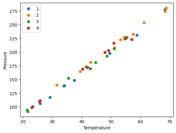
the point of this is we cannot see a visual clustering of the groups by day. That is important, because if we did it could suggest something was different that day.

Combining data sets¶

Siddhant Lambor provided from two experiments conducted to measure the properties of a worm-like micelles solution. He had carried out experiments on a rheometer to measure the viscosity of a worm-like micelles solution in a Couette cell geometry and a Cone and Plate geometry. Ideally, there should not be a difference as viscosity is intrinsic to the fluid. Analysis of this data will confirm if that is true. First, we read this data in from the two data files.

cp.xlsx Cone and plate data
couette.xlsx Couette data

couette = pd.read_excel(
    "couette.xls", sheet_name="Flow sweep - 1", header=1
)  # sheet name is case sensitive, excel file name is not

couette

	Stress	Shear rate	Viscosity	Step time	Temperature	Normal stress
0	Pa	1/s	Pa.s	s	°C	Pa
1	0.009981	0.04953	0.201504	35.1469	25.001	-0.001263
2	0.015817	0.079875	0.198028	70.1689	25.001	-0.000835
3	0.025071	0.127313	0.196926	105.253	25	-0.000913
4	0.039734	0.204094	0.194685	140.26	25	-0.001132
5	0.062977	0.327253	0.192442	175.313	25	-0.002026
6	0.099806	0.530364	0.188183	210.32	24.998	-0.002429
7	0.158165	0.875494	0.180658	245.373	25	-0.001837
8	0.250637	1.49135	0.168061	280.426	25.002	-0.001655
9	0.397131	2.64707	0.150027	315.433	25.001	-0.001889
10	0.629111	5.00904	0.125595	350.501	25.003	-0.002233
11	0.996153	10.3993	0.09579	385.508	24.996	-0.001807
12	1.57528	24.5624	0.064134	420.608	24.998	-0.001823
13	2.47652	67.2972	0.0368	455.63	25.003	-0.00182
14	3.75092	210.991	0.017778	490.668	25	-0.002939

We can drop the row at index 0, it just has the units in it. With this syntax, we have to save the resulting DataFrame back into the variable, or it will not be changed.

couette = couette.drop(0)
couette

	Stress	Shear rate	Viscosity	Step time	Temperature	Normal stress
1	0.009981	0.04953	0.201504	35.1469	25.001	-0.001263
2	0.015817	0.079875	0.198028	70.1689	25.001	-0.000835
3	0.025071	0.127313	0.196926	105.253	25	-0.000913
4	0.039734	0.204094	0.194685	140.26	25	-0.001132
5	0.062977	0.327253	0.192442	175.313	25	-0.002026
6	0.099806	0.530364	0.188183	210.32	24.998	-0.002429
7	0.158165	0.875494	0.180658	245.373	25	-0.001837
8	0.250637	1.49135	0.168061	280.426	25.002	-0.001655
9	0.397131	2.64707	0.150027	315.433	25.001	-0.001889
10	0.629111	5.00904	0.125595	350.501	25.003	-0.002233
11	0.996153	10.3993	0.09579	385.508	24.996	-0.001807
12	1.57528	24.5624	0.064134	420.608	24.998	-0.001823
13	2.47652	67.2972	0.0368	455.63	25.003	-0.00182
14	3.75092	210.991	0.017778	490.668	25	-0.002939

There is a second file called cp.xls we want to combine with this. Here, we combine the drop function all into one line.

conePlate = pd.read_excel("cp.xls", sheet_name="Flow sweep - 1", header=1).drop(0)
conePlate.head(5)

	Stress	Shear rate	Viscosity	Step time	Temperature	Normal stress
1	0.009984	0.053193	0.187693	34.9909	25	1.2658
2	0.015822	0.082	0.19295	70.0909	25.001	0.569149
3	0.025078	0.129969	0.192952	105.16	25	0.295899
4	0.039759	0.20176	0.19706	140.213	25	1.0171
5	0.062988	0.336087	0.187415	175.282	25	0.546196

For this analysis, we are only interested in the shear rate, stress and viscosity values. Let us drop the other columns. We do that by the names, and specify inplace=True, which modifies the DataFrame itself.

conePlate.drop(["Temperature", "Step time", "Normal stress"], axis=1, inplace=True)
# if we do not use inplace=True, the data frame will not be changed. It would by default create a new data frame
# and we would have to assign a different variable to capture this change.
conePlate.head(5)

	Stress	Shear rate	Viscosity
1	0.009984	0.053193	0.187693
2	0.015822	0.082	0.19295
3	0.025078	0.129969	0.192952
4	0.039759	0.20176	0.19706
5	0.062988	0.336087	0.187415

We also do that for the couette data. Here we did not use inplace=True, so we have to save the result back into the variable to get the change.

couette = couette.drop(
    ["Temperature", "Step time", "Normal stress"], axis=1
)  # without using inplace = True
couette.head(5)

	Stress	Shear rate	Viscosity
1	0.009981	0.04953	0.201504
2	0.015817	0.079875	0.198028
3	0.025071	0.127313	0.196926
4	0.039734	0.204094	0.194685
5	0.062977	0.327253	0.192442

We can see info about each DataFrame like this.

couette.info()

<class 'pandas.core.frame.DataFrame'>
RangeIndex: 14 entries, 1 to 14
Data columns (total 3 columns):
 #   Column      Non-Null Count  Dtype 
---  ------      --------------  ----- 
 0   Stress      14 non-null     object
 1   Shear rate  14 non-null     object
 2   Viscosity   14 non-null     object
dtypes: object(3)
memory usage: 468.0+ bytes

conePlate.info()

<class 'pandas.core.frame.DataFrame'>
RangeIndex: 17 entries, 1 to 17
Data columns (total 3 columns):
 #   Column      Non-Null Count  Dtype 
---  ------      --------------  ----- 
 0   Stress      17 non-null     object
 1   Shear rate  17 non-null     object
 2   Viscosity   17 non-null     object
dtypes: object(3)
memory usage: 540.0+ bytes

We could proceed to analyze the DataFrames separately, but instead, we will combine them into one DataFrame. Before doing that, we need to add a column to each one so we know which data set is which. Simply assigning a value to a new column name will do that.

couette["type"] = "couette"
couette

	Stress	Shear rate	Viscosity	type
1	0.009981	0.04953	0.201504	couette
2	0.015817	0.079875	0.198028	couette
3	0.025071	0.127313	0.196926	couette
4	0.039734	0.204094	0.194685	couette
5	0.062977	0.327253	0.192442	couette
6	0.099806	0.530364	0.188183	couette
7	0.158165	0.875494	0.180658	couette
8	0.250637	1.49135	0.168061	couette
9	0.397131	2.64707	0.150027	couette
10	0.629111	5.00904	0.125595	couette
11	0.996153	10.3993	0.09579	couette
12	1.57528	24.5624	0.064134	couette
13	2.47652	67.2972	0.0368	couette
14	3.75092	210.991	0.017778	couette

conePlate["type"] = "cone"

Now, we can combine these into a single DataFrame. This is not critical, and you can get by without it, but I want to explore the idea, and illustrate it is possible.

df = pd.concat([conePlate, couette])
df

	Stress	Shear rate	Viscosity	type
1	0.009984	0.053193	0.187693	cone
2	0.015822	0.082	0.19295	cone
3	0.025078	0.129969	0.192952	cone
4	0.039759	0.20176	0.19706	cone
5	0.062988	0.336087	0.187415	cone
6	0.09982	0.556749	0.179291	cone
7	0.15819	0.925403	0.170942	cone
8	0.250701	1.57526	0.159148	cone
9	0.397263	2.782	0.142798	cone
10	0.629346	5.16333	0.121888	cone
11	0.996863	10.4029	0.095826	cone
12	1.57768	23.6558	0.066693	cone
13	2.49053	62.5901	0.039791	cone
14	3.85502	194.265	0.019844	cone
15	5.45425	795.474	0.006857	cone
16	8.62182	2011.14	0.004287	cone
17	13.7498	3633.47	0.003784	cone
1	0.009981	0.04953	0.201504	couette
2	0.015817	0.079875	0.198028	couette
3	0.025071	0.127313	0.196926	couette
4	0.039734	0.204094	0.194685	couette
5	0.062977	0.327253	0.192442	couette
6	0.099806	0.530364	0.188183	couette
7	0.158165	0.875494	0.180658	couette
8	0.250637	1.49135	0.168061	couette
9	0.397131	2.64707	0.150027	couette
10	0.629111	5.00904	0.125595	couette
11	0.996153	10.3993	0.09579	couette
12	1.57528	24.5624	0.064134	couette
13	2.47652	67.2972	0.0368	couette
14	3.75092	210.991	0.017778	couette

Finally, we are ready for the visualization. We will group the DataFrame and then make plots for each group. Here we illustrate several new arguments, including loglog plots, secondary axes, colored tick labels, and multiple legends.

g = df.groupby("type")
ax1 = g.get_group("cone").plot(
    "Shear rate", "Viscosity", logx=True, logy=True, style="b.-", label="CP viscosity"
)

g.get_group("couette").plot(
    "Shear rate",
    "Viscosity",
    logx=True,
    logy=True,
    style="g.-",
    ax=ax1,
    label="Couette viscosity",
)

ax2 = g.get_group("cone").plot(
    "Shear rate",
    "Stress",
    secondary_y=True,
    logx=True,
    logy=True,
    style="r.-",
    ax=ax1,
    label="CP stress",
)

g.get_group("couette").plot(
    "Shear rate",
    "Stress",
    secondary_y=True,
    logx=True,
    logy=True,
    style="y.",
    ax=ax2,
    label="Couette Stress",
)

# Setting y axis labels
ax1.set_ylabel("Viscosity (Pa.s)", color="b")
[ticklabel.set_color("b") for ticklabel in ax1.get_yticklabels()]

ax2.set_ylabel("Stress (Pa)", color="r")
[ticklabel.set_color("r") for ticklabel in ax1.get_yticklabels()]

# setting legend locations
ax1.legend(loc=6)
ax2.legend(loc=7)

ax1.set_xlabel("Shear rate (1/s)")
plt.title("Comparison of Cone and Plate with Couette Cell")

Text(0.5, 1.0, 'Comparison of Cone and Plate with Couette Cell')

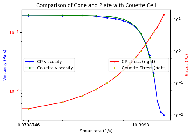
So, in fact we can see these two experiments are practically equivalent.

Data science and machine learning in science and engineering

Intermediate Pandas

Contents

Intermediate Pandas¶

Revisiting a previous example with batches of data¶

Combining data sets¶