.ipynb .pdf

repository open issue

Binder

Contents

Introduction to Pandas

Before we jump into Pandas, let us review what we have considered so far.

First, we learned how to read data from files into numpy arrays. We learned how to use variables to store that data, and to either slice the array into a few variables, or use slices themselves for something. We also learned how to make a record array that enabled us to access columns of the array by a name.

When we loaded a json file, we got a dictionary data structure, which also allowed us to access data by a name.

Second, we imported a visualization library, and made plots that used the arrays as arguments.

For “small” data sets, i.e. not too many columns, this is a perfectly reasonable thing to do. For larger datasets, however, it can be tedious to create a lot of variable names, and it is also hard to remember what is in each column.

Many tasks are pretty standard, e.g. read a data set, summarize and visualize it. It would be nice if we had a simple way to do this, with few lines of code, since those lines will be the same every time.

The Pandas library was developed to address all these issues. From the website: “pandas is a fast, powerful, flexible and easy to use open source data analysis and manipulation tool, built on top of the Python programming language.”

Review of the numpy array way

Let’s review what we learned already.

import matplotlib.pyplot as plt
import numpy as np

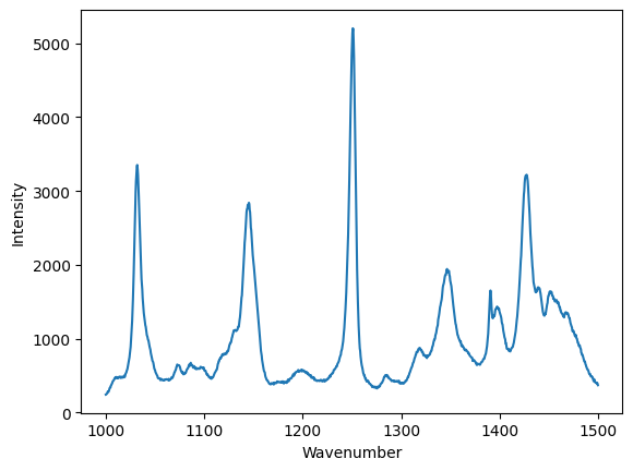
data = np.loadtxt("raman.txt")

wavenumber, intensity = data.T  # the transpose has data in rows for unpacking
ind = (wavenumber >= 1000) & (wavenumber < 1500)


plt.figure()
plt.plot(wavenumber[ind], intensity[ind])
plt.xlabel("Wavenumber")
plt.ylabel("Intensity");

Now, with Pandas

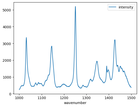
We will unpack this code shortly. For now, look how short it is to create this plot. Note that we have condensed all the code in the example above basically into three lines of code. That is pretty remarkable, but should give you some pause. We now have to learn how to use such a dense syntax!

import pandas as pd

df = pd.read_csv(
    "raman.txt", delimiter="\t", index_col=0, names=["wavenumber", "intensity"]
)
df[(df.index >= 1000) & (df.index < 1500)].plot();

And to summarize.

df.describe()

	intensity
count	7620.000000
mean	558.388392
std	982.659031
min	77.104279
25%	113.666535
50%	219.409340
75%	552.632848
max	15275.059000

What is the benefit of this dense syntax? Because it is so short, it is faster to type (at least, when you know what to type). That means it is also faster for you to read.

The downside is that it is like learning a whole new language within Python, and a new mental model for how the data is stored and accessed. You have to decide if it is worthwhile doing that. If you do this a lot, it is probably worthwhile.

Pandas

The main object we will work with is called a DataFrame.

type(df)

pandas.core.frame.DataFrame

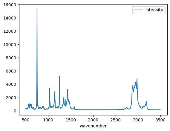
Jupyter notebooks can show you a fancy rendering of your dataframe.

df

	intensity
wavenumber
500.00000	294.378690
500.39374	288.922000
500.78751	286.066220
501.18124	275.222840
501.57501	275.119380
...	...
3498.42500	86.151878
3498.81880	85.178947
3499.21240	87.969734
3499.60620	83.638931
3500.00000	84.009064

7620 rows × 1 columns

The dataframe combines a few ideas we used from arrays and dictionaries. First, we can access a column by name. When we do this, we get a Series object.

type(df["intensity"])

pandas.core.series.Series

You can extract the values into a numpy array like this.

df["intensity"].values

array([294.37869 , 288.922   , 286.06622 , ...,  87.969734,  83.638931,
        84.009064])

A Series (and DataFrame) are like numpy arrays in some ways, and different in others. Suppose we want to see the first five entries of the intensity. If we want to use integer-based indexing like we have so far, you have to use the iloc attribute on the series like this. iloc is for integer location.

df["intensity"].iloc[0:5]

wavenumber
500.00000    294.37869
500.39374    288.92200
500.78751    286.06622
501.18124    275.22284
501.57501    275.11938
Name: intensity, dtype: float64

What about the wavenumbers? These are called the index of the dataframe.

df.index

Index([    500.0, 500.39374, 500.78751, 501.18124, 501.57501, 501.96875,
       502.36252, 502.75626, 503.15002, 503.54376,
       ...
       3496.4563, 3496.8501, 3497.2437, 3497.6375, 3498.0313,  3498.425,
       3498.8188, 3499.2124, 3499.6062,    3500.0],
      dtype='float64', name='wavenumber', length=7620)

You can index the index with integers as you can with an array.

df.index[0:5]

Index([500.0, 500.39374, 500.78751, 501.18124, 501.57501], dtype='float64', name='wavenumber')

Finally, you can combine these so that you index a column with a slice of the index like this.

df["intensity"][df.index[0:5]]

wavenumber
500.00000    294.37869
500.39374    288.92200
500.78751    286.06622
501.18124    275.22284
501.57501    275.11938
Name: intensity, dtype: float64

In summary, we can think of a dataframe as a hybrid array/dictionary where we have an index which is like the independent variable, and a set of columns that are like dependent variables. You can access the columns like a dictionary.

Dataframes and visualization

Dataframes also provide easy access to visualization. The simplest method is to just call the plot method on a dataframe. Note this automatically makes the plot with labels and a legend. If there are many columns, you will have a curve for each one of them. We will see that later.

df.plot();

Reading data in Pandas

Let’s get back to how we got the data into Pandas. Let’s retrieve the data file we used before with several columns in it.

fname = "p-t.dat"
url = "https://www.itl.nist.gov/div898/handbook/datasets/MODEL-4_4_4.DAT"

import urllib.request

urllib.request.urlretrieve(url, fname);

Let’s refresh our memory of what is in this file:

! head p-t.dat

 Run          Ambient                            Fitted

Order  Day  Temperature  Temperature  Pressure    Value    Residual

 1      1      23.820      54.749      225.066   222.920     2.146

 2      1      24.120      23.323      100.331    99.411     0.920

 3      1      23.434      58.775      230.863   238.744    -7.881

 4      1      23.993      25.854      106.160   109.359    -3.199

 5      1      23.375      68.297      277.502   276.165     1.336

 6      1      23.233      37.481      148.314   155.056    -6.741

 7      1      24.162      49.542      197.562   202.456    -4.895

 8      1      23.667      34.101      138.537   141.770    -3.232

We use Pandas.read_csv to read this, similar to how we used numpy.loadtxt. It also takes a lot of arguments to fine-tune the output. We use spaces as the delimiter here. '\s+' is a regular expression for multiple spaces. We still skip two rows, and we have to manually define the column names. We do not specify an index column here, we get a default one based on integers. Pandas is smart enough to recognize the first two columns are integers, so we do not have to do anything special here.

df = pd.read_csv(
    "p-t.dat",
    delimiter="\s+",
    skiprows=2,
    names=[
        "Run order",
        "Day",
        "Ambient Temperature",
        "Temperature",
        "Pressure",
        "Fitted Value",
        "Residual",
    ],
)
df

	Run order	Day	Ambient Temperature	Temperature	Pressure	Fitted Value	Residual
0	1	1	23.820	54.749	225.066	222.920	2.146
1	2	1	24.120	23.323	100.331	99.411	0.920
2	3	1	23.434	58.775	230.863	238.744	-7.881
3	4	1	23.993	25.854	106.160	109.359	-3.199
4	5	1	23.375	68.297	277.502	276.165	1.336
5	6	1	23.233	37.481	148.314	155.056	-6.741
6	7	1	24.162	49.542	197.562	202.456	-4.895
7	8	1	23.667	34.101	138.537	141.770	-3.232
8	9	1	24.056	33.901	137.969	140.983	-3.014
9	10	1	22.786	29.242	117.410	122.674	-5.263
10	11	2	23.785	39.506	164.442	163.013	1.429
11	12	2	22.987	43.004	181.044	176.759	4.285
12	13	2	23.799	53.226	222.179	216.933	5.246
13	14	2	23.661	54.467	227.010	221.813	5.198
14	15	2	23.852	57.549	232.496	233.925	-1.429
15	16	2	23.379	61.204	253.557	248.288	5.269
16	17	2	24.146	31.489	139.894	131.506	8.388
17	18	2	24.187	68.476	273.931	276.871	-2.940
18	19	2	24.159	51.144	207.969	208.753	-0.784
19	20	2	23.803	68.774	280.205	278.040	2.165
20	21	3	24.381	55.350	227.060	225.282	1.779
21	22	3	24.027	44.692	180.605	183.396	-2.791
22	23	3	24.342	50.995	206.229	208.167	-1.938
23	24	3	23.670	21.602	91.464	92.649	-1.186
24	25	3	24.246	54.673	223.869	222.622	1.247
25	26	3	25.082	41.449	172.910	170.651	2.259
26	27	3	24.575	35.451	152.073	147.075	4.998
27	28	3	23.803	42.989	169.427	176.703	-7.276
28	29	3	24.660	48.599	192.561	198.748	-6.188
29	30	3	24.097	21.448	94.448	92.042	2.406
30	31	4	22.816	56.982	222.794	231.697	-8.902
31	32	4	24.167	47.901	199.003	196.008	2.996
32	33	4	22.712	40.285	168.668	166.077	2.592
33	34	4	23.611	25.609	109.387	108.397	0.990
34	35	4	23.354	22.971	98.445	98.029	0.416
35	36	4	23.669	25.838	110.987	109.295	1.692
36	37	4	23.965	49.127	202.662	200.826	1.835
37	38	4	22.917	54.936	224.773	223.653	1.120
38	39	4	23.546	50.917	216.058	207.859	8.199
39	40	4	24.450	41.976	171.469	172.720	-1.251

The default plot is not that nice.

df.plot();

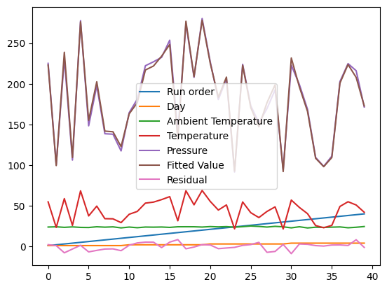
The default is to plot each column vs the index, which is not that helpful for us. Say we just want to plot the pressure vs. the temperature.

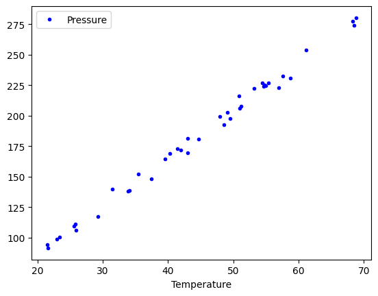
df.plot(x="Temperature", y="Pressure", style="b.");

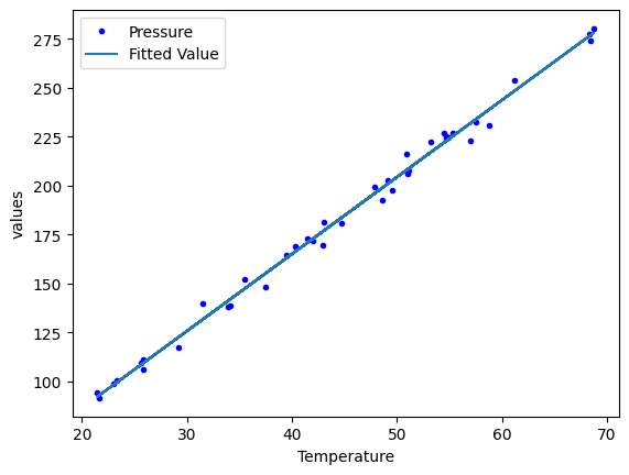
We can add multiple plots to a figure, but we have to tell the subsequent calls which axes to put them on. To do that, save the first one, and pass it as an argument in subsequent plots. That also allows you to fine-tune the plot appearance, e.g. add a y-label. See the matplotlib documentation to learn how to set all of these.

p1 = df.plot(x="Temperature", y="Pressure", style="b.")
df.plot(x="Temperature", y="Fitted Value", ax=p1)

p1.set_ylabel("values");

It is a reasonable question to ask if this is simpler than what we did before using arrays, variables and plotting commands. Dataframes are increasingly common in data science, and are the data structure used in many data science/machine learning projects.

Another real-life example

LAMMPS is a molecular simulation code used to run molecular dynamics. It outputs a text file that is somewhat challenging to read. There are variable numbers of time steps that depend on how the simulation was setup.

Start by downloading and opening this file. It is a molecular dynamics trajectory at constant volume, where the pressure, temperature and energy fluctuate.

Open this file log1.lammpsto get a sense for what is in it. The data starts around:

timestep 0.005
run ${runSteps}
run 500000
Per MPI rank memory allocation (min/avg/max) = 4.427 | 4.427 | 4.427 Mbytes
Step v_mytime Temp Press Volume PotEng TotEng v_pxy v_pxz v_pyz v_v11 v_v22 v_v33 CPU
       0            0         1025    601.28429    8894.6478   -1566.6216   -1500.5083    2065.6285    1713.4095    203.00499 1.3408976e-05 9.2260011e-06 1.2951038e-07            0 w

And it ends around this line.

  500000         2500    978.62359   -2100.7614    8894.6478   -1570.5382   -1507.4162   -252.80665    614.87398    939.65393 0.00045263648 0.00043970796 0.00044228719    1288.0233
Loop time of 1288.02 on 1 procs for 500000 steps with 500 atoms

Our job is to figure out where those lines are so we can read them into Pandas. There are many ways to do this, but we will stick with a pure Python way. The strategy is to search for the lines, and keep track of their positions.

start, stop = None, None
with open("log1.lammps") as f:
    for i, line in enumerate(f):
        if line.startswith("Step v_mytime"):
            start = i
        if line.startswith("Loop time of "):
            stop = i - 1  # stop on the previous line
            break
start, stop

(69, 2570)

This gets tricky. We want to skip the rows up to the starting line. At that point, the line numbers restart as far as Pandas is concerned, so the header is in line 0 then, and the number of rows to read is defined by the stop line minus the start line. The values are separated by multiple spaces, so we use a pattern to indicate multiple spaces. Finally, we prevent the first column from being the index column by setting index_col to be False. See https://pandas.pydata.org/pandas-docs/stable/reference/api/pandas.read_csv.html>for all the details.

df = pd.read_csv(
    "log1.lammps",
    skiprows=start,
    header=0,
    nrows=stop - start,
    delimiter="\s+",
    index_col=False,
)
df

/tmp/ipykernel_2193/86227813.py:1: ParserWarning: Length of header or names does not match length of data. This leads to a loss of data with index_col=False.
  df = pd.read_csv(

	Step	v_mytime	Temp	Press	Volume	PotEng	TotEng	v_pxy	v_pxz	v_pyz	v_v11	v_v22	v_v33	CPU
0	0	0	1025.00000	601.28429	8894.6478	-1566.6216	-1500.5083	2065.62850	1713.409500	203.00499	0.000013	0.000009	1.295104e-07	0.000000
1	200	1	1045.85100	-1974.43580	8894.6478	-1569.6934	-1502.2352	2530.16720	-2203.376800	-2193.88770	0.000423	-0.000564	9.109558e-04	0.505391
2	400	2	1050.44480	2974.54030	8894.6478	-1564.3755	-1496.6210	1446.73930	637.829780	1794.70610	0.001115	0.000125	4.583668e-04	1.018666
3	600	3	1071.37780	2386.37510	8894.6478	-1566.4325	-1497.3278	599.73943	-462.748090	558.54192	0.000766	0.000387	3.082071e-04	1.532061
4	800	4	1055.52810	-661.78795	8894.6478	-1569.3172	-1501.2348	1775.43870	-1551.263500	-493.01032	0.000569	0.000380	2.913082e-04	2.051839
...	...	...	...	...	...	...	...	...	...	...	...	...	...	...
2496	499200	2496	977.95894	-1747.91220	8894.6478	-1570.0162	-1506.9370	1411.85600	1154.883400	-2265.50500	0.000452	0.000440	4.424962e-04	1285.960300
2497	499400	2497	1066.50870	-77.15260	8894.6478	-1568.3816	-1499.5910	4071.88400	3847.295900	-1279.02860	0.000452	0.000440	4.428113e-04	1286.474100
2498	499600	2498	1052.18860	1958.97410	8894.6478	-1565.8013	-1497.9343	-2152.54460	925.775780	-1162.76120	0.000453	0.000439	4.427215e-04	1286.987000
2499	499800	2499	1057.30140	-1709.95670	8894.6478	-1570.6800	-1502.4832	-1530.34090	-71.479217	731.44735	0.000453	0.000440	4.423706e-04	1287.503200
2500	500000	2500	978.62359	-2100.76140	8894.6478	-1570.5382	-1507.4162	-252.80665	614.873980	939.65393	0.000453	0.000440	4.422872e-04	1288.023300

2501 rows × 14 columns

Visualizing the data

Plot a column

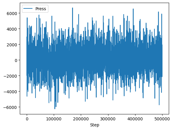
The effort was worth it though; look how easy it is to plot the data!

df.plot(x="Step", y="Press");

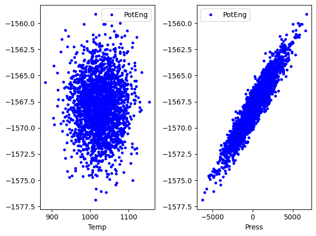
import matplotlib.pyplot as plt

fig, (ax0, ax1) = plt.subplots(1, 2)
df.plot(x="Temp", y="PotEng", style="b.", ax=ax0)
df.plot(x="Press", y="PotEng", style="b.", ax=ax1)
plt.tight_layout();

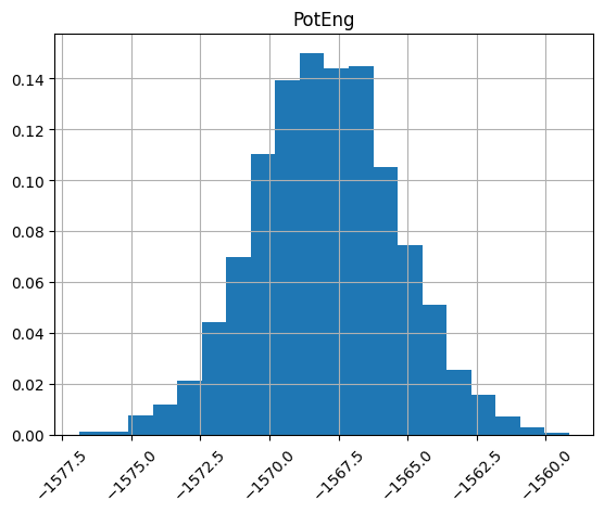
Plot distributions of a column

We can look at histograms of properties as easily.

df.hist("PotEng", xrot=45, bins=20, density=True);

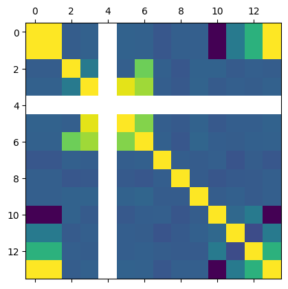
Plot column correlations

This is just the beginning of using Pandas. Suppose we want to see which columns are correlated (https://pandas.pydata.org/pandas-docs/stable/reference/api/pandas.DataFrame.corr.html). With variables this would be tedious.

plt.matshow(df.corr());

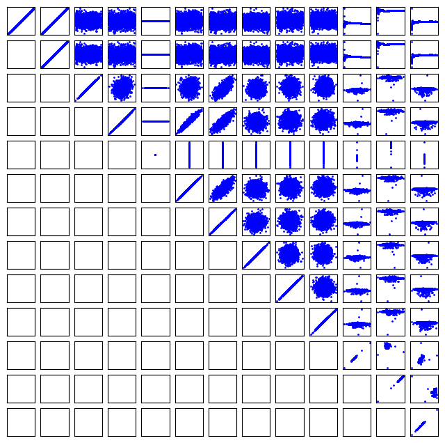
It can be helpful to see what these correlations mean. Here we plot all the columns against each other. Note, it is not possible to plot a column against itself with Pandas (I think this is a bug https://github.com/pandas-dev/pandas/issues/22088), so here I use matplotlib functions for the plotting. This should be symmetric, so I only plot the upper triangle.

keys = df.keys()

fig, axs = plt.subplots(13, 13)
fig.set_size_inches((8, 8))
for i in range(13):
    for j in range(i, 13):
        axs[i, j].plot(df[keys[i]], df[keys[j]], "b.", ms=2)
        # remove axes so it is easier to read
        axs[i, j].axes.get_xaxis().set_visible(False)
        axs[i, j].axes.get_yaxis().set_visible(False)
        axs[j, i].axes.get_xaxis().set_visible(False)
        axs[j, i].axes.get_yaxis().set_visible(False)

Getting parts of a Pandas DataFrame

We have seen how to get a column from a DataFrame like this:

df["Press"]

0        601.28429
1      -1974.43580
2       2974.54030
3       2386.37510
4       -661.78795
           ...    
2496   -1747.91220
2497     -77.15260
2498    1958.97410
2499   -1709.95670
2500   -2100.76140
Name: Press, Length: 2501, dtype: float64

In this context, the DataFrame is acting like a dictionary. You can get a few columns by using a list of column names.

df[["Press", "PotEng"]]

	Press	PotEng
0	601.28429	-1566.6216
1	-1974.43580	-1569.6934
2	2974.54030	-1564.3755
3	2386.37510	-1566.4325
4	-661.78795	-1569.3172
...	...	...
2496	-1747.91220	-1570.0162
2497	-77.15260	-1568.3816
2498	1958.97410	-1565.8013
2499	-1709.95670	-1570.6800
2500	-2100.76140	-1570.5382

2501 rows × 2 columns

What about a row? This is what we would have done with a numpy array, but it just doesn’t work here.

Error

You get a KeyError here.

df[0]

---------------------------------------------------------------------------
KeyError                                  Traceback (most recent call last)
File /opt/hostedtoolcache/Python/3.8.17/x64/lib/python3.8/site-packages/pandas/core/indexes/base.py:3652, in Index.get_loc(self, key)
   3651 try:
-> 3652     return self._engine.get_loc(casted_key)
   3653 except KeyError as err:

File /opt/hostedtoolcache/Python/3.8.17/x64/lib/python3.8/site-packages/pandas/_libs/index.pyx:147, in pandas._libs.index.IndexEngine.get_loc()

File /opt/hostedtoolcache/Python/3.8.17/x64/lib/python3.8/site-packages/pandas/_libs/index.pyx:176, in pandas._libs.index.IndexEngine.get_loc()

File pandas/_libs/hashtable_class_helper.pxi:7080, in pandas._libs.hashtable.PyObjectHashTable.get_item()

File pandas/_libs/hashtable_class_helper.pxi:7088, in pandas._libs.hashtable.PyObjectHashTable.get_item()

KeyError: 0

The above exception was the direct cause of the following exception:

KeyError                                  Traceback (most recent call last)
Cell In[28], line 1
----> 1 df[0]

File /opt/hostedtoolcache/Python/3.8.17/x64/lib/python3.8/site-packages/pandas/core/frame.py:3761, in DataFrame.__getitem__(self, key)
   3759 if self.columns.nlevels > 1:
   3760     return self._getitem_multilevel(key)
-> 3761 indexer = self.columns.get_loc(key)
   3762 if is_integer(indexer):
   3763     indexer = [indexer]

File /opt/hostedtoolcache/Python/3.8.17/x64/lib/python3.8/site-packages/pandas/core/indexes/base.py:3654, in Index.get_loc(self, key)
   3652     return self._engine.get_loc(casted_key)
   3653 except KeyError as err:
-> 3654     raise KeyError(key) from err
   3655 except TypeError:
   3656     # If we have a listlike key, _check_indexing_error will raise
   3657     #  InvalidIndexError. Otherwise we fall through and re-raise
   3658     #  the TypeError.
   3659     self._check_indexing_error(key)

KeyError: 0

The problem is that as a dictionary, the keys are for the columns.

df.keys()

Index(['Step', 'v_mytime', 'Temp', 'Press', 'Volume', 'PotEng', 'TotEng',
       'v_pxy', 'v_pxz', 'v_pyz', 'v_v11', 'v_v22', 'v_v33', 'CPU'],
      dtype='object')

One way to get the rows by their integer index is to use the integer location attribute for a row.

df.iloc[0]

Step        0.000000e+00
v_mytime    0.000000e+00
Temp        1.025000e+03
Press       6.012843e+02
Volume      8.894648e+03
PotEng     -1.566622e+03
TotEng     -1.500508e+03
v_pxy       2.065628e+03
v_pxz       1.713409e+03
v_pyz       2.030050e+02
v_v11       1.340898e-05
v_v22       9.226001e-06
v_v33       1.295104e-07
CPU         0.000000e+00
Name: 0, dtype: float64

We can use slices on this.

df.iloc[0:5]

	Step	v_mytime	Temp	Press	Volume	PotEng	TotEng	v_pxy	v_pxz	v_pyz	v_v11	v_v22	v_v33	CPU
0	0	0	1025.0000	601.28429	8894.6478	-1566.6216	-1500.5083	2065.62850	1713.40950	203.00499	0.000013	0.000009	1.295104e-07	0.000000
1	200	1	1045.8510	-1974.43580	8894.6478	-1569.6934	-1502.2352	2530.16720	-2203.37680	-2193.88770	0.000423	-0.000564	9.109558e-04	0.505391
2	400	2	1050.4448	2974.54030	8894.6478	-1564.3755	-1496.6210	1446.73930	637.82978	1794.70610	0.001115	0.000125	4.583668e-04	1.018666
3	600	3	1071.3778	2386.37510	8894.6478	-1566.4325	-1497.3278	599.73943	-462.74809	558.54192	0.000766	0.000387	3.082071e-04	1.532061
4	800	4	1055.5281	-661.78795	8894.6478	-1569.3172	-1501.2348	1775.43870	-1551.26350	-493.01032	0.000569	0.000380	2.913082e-04	2.051839

This example may be a little confusing, because our index does include 0, so we can in this case also use the row label with the location attribute. You can use any value in the index for this.

df.index

RangeIndex(start=0, stop=2501, step=1)

df.loc[0]

Step        0.000000e+00
v_mytime    0.000000e+00
Temp        1.025000e+03
Press       6.012843e+02
Volume      8.894648e+03
PotEng     -1.566622e+03
TotEng     -1.500508e+03
v_pxy       2.065628e+03
v_pxz       1.713409e+03
v_pyz       2.030050e+02
v_v11       1.340898e-05
v_v22       9.226001e-06
v_v33       1.295104e-07
CPU         0.000000e+00
Name: 0, dtype: float64

We can access the first five rows like this.

df.loc[0:4]

	Step	v_mytime	Temp	Press	Volume	PotEng	TotEng	v_pxy	v_pxz	v_pyz	v_v11	v_v22	v_v33	CPU
0	0	0	1025.0000	601.28429	8894.6478	-1566.6216	-1500.5083	2065.62850	1713.40950	203.00499	0.000013	0.000009	1.295104e-07	0.000000
1	200	1	1045.8510	-1974.43580	8894.6478	-1569.6934	-1502.2352	2530.16720	-2203.37680	-2193.88770	0.000423	-0.000564	9.109558e-04	0.505391
2	400	2	1050.4448	2974.54030	8894.6478	-1564.3755	-1496.6210	1446.73930	637.82978	1794.70610	0.001115	0.000125	4.583668e-04	1.018666
3	600	3	1071.3778	2386.37510	8894.6478	-1566.4325	-1497.3278	599.73943	-462.74809	558.54192	0.000766	0.000387	3.082071e-04	1.532061
4	800	4	1055.5281	-661.78795	8894.6478	-1569.3172	-1501.2348	1775.43870	-1551.26350	-493.01032	0.000569	0.000380	2.913082e-04	2.051839

And a slice of a column like this.

df.loc[0:4, "Press"]

0     601.28429
1   -1974.43580
2    2974.54030
3    2386.37510
4    -661.78795
Name: Press, dtype: float64

We can access a value in a row and column with the at function on a DataFrame.

df.at[2, "Press"]

2974.5403

Or if you know the row and column numbers you can use iat.

df.iat[2, 3]

2974.5403

Operating on columns in the DataFrame

Some functions just work across the columns. For example, DataFrames have statistics functions like this.

df.mean()

Step        250000.000000
v_mytime      1250.000000
Temp          1025.136938
Press          188.035304
Volume        8894.647800
PotEng       -1567.935373
TotEng       -1501.813207
v_pxy           16.669575
v_pxz           -4.852837
v_pyz           14.175372
v_v11            0.000465
v_v22            0.000429
v_v33            0.000428
CPU            644.103768
dtype: float64

We should tread carefully with other functions that work on arrays. For example consider this example that computes the mean of an entire array.

a = np.array([[1, 1, 1], [2, 2, 2]])
np.mean(a)

1.5

It does not do the same thing on a DataFrame. The index and column labels are preserved with numpy functions.

import numpy as np

np.mean(df)  # takes mean along axis 0

18497.01204734716

np.max(df)

500000.0

np.exp(df)

/opt/hostedtoolcache/Python/3.8.17/x64/lib/python3.8/site-packages/pandas/core/internals/blocks.py:329: RuntimeWarning: overflow encountered in exp
  result = func(self.values, **kwargs)

	Step	v_mytime	Temp	Press	Volume	PotEng	TotEng	v_pxy	v_pxz	v_pyz	v_v11	v_v22	v_v33	CPU
0	1.000000e+00	1.000000	inf	1.362854e+261	inf	0.0	0.0	inf	inf	1.458636e+88	1.000013	1.000009	1.000000	1.000000
1	7.225974e+86	2.718282	inf	0.000000e+00	inf	0.0	0.0	inf	0.000000e+00	0.000000e+00	1.000423	0.999436	1.000911	1.657634
2	5.221470e+173	7.389056	inf	inf	inf	0.0	0.0	inf	1.013804e+277	inf	1.001116	1.000125	1.000458	2.769498
3	3.773020e+260	20.085537	inf	inf	inf	0.0	0.0	2.907536e+260	1.074133e-201	3.729699e+242	1.000766	1.000387	1.000308	4.627705
4	inf	54.598150	inf	3.882801e-288	inf	0.0	0.0	inf	0.000000e+00	7.732831e-215	1.000569	1.000380	1.000291	7.782200
...	...	...	...	...	...	...	...	...	...	...	...	...	...	...
2496	inf	inf	inf	0.000000e+00	inf	0.0	0.0	inf	inf	0.000000e+00	1.000452	1.000440	1.000443	inf
2497	inf	inf	inf	3.112086e-34	inf	0.0	0.0	inf	inf	0.000000e+00	1.000452	1.000440	1.000443	inf
2498	inf	inf	inf	inf	inf	0.0	0.0	0.000000e+00	inf	0.000000e+00	1.000453	1.000439	1.000443	inf
2499	inf	inf	inf	0.000000e+00	inf	0.0	0.0	0.000000e+00	9.056711e-32	inf	1.000453	1.000440	1.000442	inf
2500	inf	inf	inf	0.000000e+00	inf	0.0	0.0	1.612378e-110	1.087368e+267	inf	1.000453	1.000440	1.000442	inf

2501 rows × 14 columns

2 * df

	Step	v_mytime	Temp	Press	Volume	PotEng	TotEng	v_pxy	v_pxz	v_pyz	v_v11	v_v22	v_v33	CPU
0	0	0	2050.00000	1202.56858	17789.2956	-3133.2432	-3001.0166	4131.25700	3426.819000	406.00998	0.000027	0.000018	2.590208e-07	0.000000
1	400	2	2091.70200	-3948.87160	17789.2956	-3139.3868	-3004.4704	5060.33440	-4406.753600	-4387.77540	0.000846	-0.001128	1.821912e-03	1.010782
2	800	4	2100.88960	5949.08060	17789.2956	-3128.7510	-2993.2420	2893.47860	1275.659560	3589.41220	0.002231	0.000249	9.167335e-04	2.037332
3	1200	6	2142.75560	4772.75020	17789.2956	-3132.8650	-2994.6556	1199.47886	-925.496180	1117.08384	0.001531	0.000774	6.164143e-04	3.064122
4	1600	8	2111.05620	-1323.57590	17789.2956	-3138.6344	-3002.4696	3550.87740	-3102.527000	-986.02064	0.001137	0.000760	5.826165e-04	4.103678
...	...	...	...	...	...	...	...	...	...	...	...	...	...	...
2496	998400	4992	1955.91788	-3495.82440	17789.2956	-3140.0324	-3013.8740	2823.71200	2309.766800	-4531.01000	0.000905	0.000880	8.849924e-04	2571.920600
2497	998800	4994	2133.01740	-154.30520	17789.2956	-3136.7632	-2999.1820	8143.76800	7694.591800	-2558.05720	0.000905	0.000879	8.856225e-04	2572.948200
2498	999200	4996	2104.37720	3917.94820	17789.2956	-3131.6026	-2995.8686	-4305.08920	1851.551560	-2325.52240	0.000906	0.000879	8.854430e-04	2573.974000
2499	999600	4998	2114.60280	-3419.91340	17789.2956	-3141.3600	-3004.9664	-3060.68180	-142.958434	1462.89470	0.000905	0.000879	8.847412e-04	2575.006400
2500	1000000	5000	1957.24718	-4201.52280	17789.2956	-3141.0764	-3014.8324	-505.61330	1229.747960	1879.30786	0.000905	0.000879	8.845744e-04	2576.046600

2501 rows × 14 columns

We can apply a function to the DataFrame. The default is the columns (axis=0). Either way, we get a new DataFrame.

def minmax(roworcolumn):
    return np.min(roworcolumn), np.max(roworcolumn)


df.apply(minmax)

	Step	v_mytime	Temp	Press	Volume	PotEng	TotEng	v_pxy	v_pxz	v_pyz	v_v11	v_v22	v_v33	CPU
0	0	0	883.05875	-6247.6768	8894.6478	-1576.8745	-1513.6955	-6747.6227	-7547.8097	-7509.4468	0.000013	-0.000564	1.295104e-07	0.0000
1	500000	2500	1154.17900	6673.7634	8894.6478	-1559.1555	-1488.9586	7428.1767	6523.4548	6229.5043	0.001115	0.000531	9.109558e-04	1288.0233

Here we analyze across the rows.

df.apply(minmax, axis=1)

0       (-1566.6216, 8894.6478)
1       (-2203.3768, 8894.6478)
2       (-1564.3755, 8894.6478)
3       (-1566.4325, 8894.6478)
4       (-1569.3172, 8894.6478)
                 ...           
2496      (-2265.505, 499200.0)
2497     (-1568.3816, 499400.0)
2498     (-2152.5446, 499600.0)
2499     (-1709.9567, 499800.0)
2500     (-2100.7614, 500000.0)
Length: 2501, dtype: object

Summary

Pandas is a multipurpose data science tool. In many ways it is like a numpy array, and in many ways it is different. In some ways it is like a dictionary.

The similarities include the ability to do some indexing and slicing. This is only a partial similarity though.

The differences include integrated plotting.

previous

Introduction to data files

next

Intermediate Pandas