New Publication - An Inverse Mapping Approach for Process Systems Engineering Using Automatic Differentiation and the Implicit Function Theorem

| categories: news, publication | tags:

Solving inverse problems, where we know what outputs we want from a model and seek the inputs that provide them, is a difficult task. A conventional approach to this problem is to use a nonlinear program (NLP) solver to iteratively find the inputs for a specific output. If you seek a desired output space, then you must solve the NLP many times to map out the corresponding input space. This is often expensive, and tedious to perform. In this work, we demonstrate a new approach to solving this problem that avoids the NLP formulation, and is faster. The idea is simple; we compute a system of differential equations that maps how the input space changes with the output space. Then from a single known point we can integrate a path in the output space to automatically trace the corresponding path in the input space! We compute the system of differential equations using automatic differentiation, and the implicit derivative theorem. We show two examples of this using a steady state continuously stirred tank reactor, which is a set of nonlinear algebraic equations that define the output space from input variables, and another plug flow reactor where the output space is defined by a set of differential equations that must be numerically integrated. In both cases we use automatic differentiation to define the system of ODEs that relate outputs and inputs, and show that the path integration method developed here is as accurate and faster than even the best NLP approach. The idea in this paper is general and applicable to many other systems, not just chemical reactors.

@article{alves-2023,
  author =       {Alves, Victor and Kitchin, John R. and Lima, Fernando V.},
  title =        {An inverse mapping approach for process systems engineering
                  using automatic differentiation and the implicit function
                  theorem},
  journal =      {AIChE Journal},
  year =         2023,
  volume =       {n/a},
  number =       {n/a},
  pages =        {e18119},
  keywords =     {automatic differentiation, implicit function theorem, inverse
                  mapping, inverse problems, process systems engineering},
  doi =          {10.1002/aic.18119},
  url =
                  {https://aiche.onlinelibrary.wiley.com/doi/abs/10.1002/aic.18119}
}

Copyright (C) 2023 by John Kitchin. See the License for information about copying.

org-mode source

Org-mode version = 9.5.5

Discuss on Twitter

New publication - WhereWulff A Semiautonomous Workflow for Systematic Catalyst Surface Reactivity under Reaction Conditions

| categories: news, publication | tags:

Suppose you want to explore metal oxides as potential water oxidation electrocatalysts. There are many steps to do this. You can use databases of materials to get compositions and structures, but for each one you have to determine the ground state structure, including magnetic states, for each bulk structure, and filter out bulk materials that are not stable under water oxidation conditions. Then, using the remaining structures you have to construct slabs and determine which surfaces are likely to be stable, and most relevant. After that you have to compute adsorption energies on those surfaces to see which surfaces have the most relevant reactivity (while also being stable). This results in hundreds to thousands of calculations that depend on each other in important ways. It is very useful to use software workflow tools to facilitate and manage this process. In this paper we develop a workflow like this for exploring metal oxides for water oxidation. The software is open source and available at https://github.com/ulissigroup/wherewulff.

The paper is free to read for 6 months at https://pubs.acs.org/doi/10.1021/acs.jcim.3c00142.

@article{sanspeur-2023,
  author = {Rohan Yuri Sanspeur and Javier Heras-Domingo and John R. Kitchin and Zachary Ulissi},
  title = {wherewulff: a Semiautonomous Workflow for Systematic Catalyst Surface Reactivity Under Reaction Conditions},
  journal = {Journal of Chemical Information and Modeling},
  volume = {nil},
  number = {nil},
  pages = {nil},
  year = {2023},
  doi = {10.1021/acs.jcim.3c00142},
  url = {http://dx.doi.org/10.1021/acs.jcim.3c00142},
  DATE_ADDED = {Sun Apr 16 09:17:23 2023},
}

Copyright (C) 2023 by John Kitchin. See the License for information about copying.

org-mode source

Org-mode version = 9.5.5

Discuss on Twitter

New publication - High throughput discovery of ternary Cu-Fe-Ru alloy catalysts for photo-driven hydrogen production

| categories: news, publication | tags:

Finding new ways to make hydrogen with renewable energy and renewable feedstocks using earth abundant materials remains a challenge in catalysis today. Metal nanoparticles are common heterogeneous catalysts for hydrogen production, and their properties can often be improved by using multiple metals at a time. In this work we show a high-throughput experimental approach to discovering a ternary alloy catalyst containing earth abundant metals that is more active at producing hydrogen than any of the pure metals it is made of. It a surprising discovery because these metals are not typically miscible, and they do not form a well characterized material, but rather a distribution of particle sizes and compositions.

@article{bhat-2023-high-throug,
  author = {Maya Bhat and Zoe C Simon and Savannah Talledo and Riti Sen and Jacob H. Smith and Stefan Bernhard and Jill E Millstone and John R Kitchin},
  title = {High Throughput Discovery of Ternary Cu-Fe-Ru Alloy Catalysts for Photo-Driven Hydrogen Production},
  journal = {Reaction Chemistry \& Engineering},
  volume = {nil},
  number = {nil},
  pages = {nil},
  year = {2023},
  doi = {10.1039/d3re00059a},
  url = {http://dx.doi.org/10.1039/D3RE00059A},
  DATE_ADDED = {Sat Apr 15 07:55:55 2023},
}

Copyright (C) 2023 by John Kitchin. See the License for information about copying.

org-mode source

Org-mode version = 9.5.5

Discuss on Twitter

MS Word comments from org-mode

| categories: orgmode, docx | tags:

TL;DR:

Today I learned you can make a Word document from org-mode with Word comments in them. This could be useful when working with collaborators maybe. The gist is you use html for the comment, then export to markdown or html, then let pandoc convert those to docx. A comment in HTML looks like this:

<span class="comment-start" author="jkitchin">Comment text</span>The text being commented on <span class="comment-end"></span> 

Let's wrap that in a link for convenience. I use a full display so it is easy to see the comment. I only export the comment for markdown and html export, for everything else we just use the path. We somewhat abuse the link syntax here by using the path for the text to comment on, and the description for the comment.

(org-link-set-parameters
 "comment"
 :export (lambda (path desc backend)
           (if (member backend '(md html))
               (format "<span class=\"comment-start\" author=\"%s\">%s</span>%s<span class=\"comment-end\"></span>"
                       (user-full-name)
                       desc
                       path)
             ;; ignore for other backends and just use path
             path))
 :display 'full
 :face '(:foreground "orange"))                  

Now, we use it like this This is the commentThis is the text commented on.

In org-mode it looks like:

To get the Word doc, we need some code that first exports to Markdown, and then calls pandoc to convert that to docx. Here is my solution to that. Usually you would put this in a subsection tagged with :noexport: but I show it here to see it. Running this block generates the docx file and opens it. Here I also leverage org-ref to get some citations and cross-references.

(require 'org-ref-refproc)
(let* ((org-export-before-parsing-hook '(org-ref-cite-natmove ;; do this first
                                        org-ref-csl-preprocess-buffer
                                        org-ref-refproc))
       (md (org-md-export-to-markdown))
       (docx (concat (file-name-sans-extension md) ".docx")))
  (shell-command (format "pandoc -s %s -o %s" md docx))
  (org-open-file docx '(16)))

The result looks like this in MS Word:

How a comment looks in Word.

That is pretty remarkable. There are some limitations in Markdown, e.g. I find the tables don't look good, not all equations are converted, some cross-references are off. Next we add some more org-features and try the export with HTML.

1. export features for test

Test cross-references, references, equations, etc…

Aliquam erat volutpat (Fig. fig-2). Nunc eleifend leo vitae magna. In id erat non orci commodo lobortis. Proin neque massa, cursus ut, gravida ut, lobortis eget, lacus. Sed diam. Praesent fermentum tempor tellus. Nullam tempus &yang-2022-evaluat-degree. Mauris ac felis vel velit tristique imperdiet. Donec at pede. Etiam vel neque nec dui dignissim bibendum. Vivamus id enim. Phasellus neque orci, porta a, aliquet quis in Table tab-1, semper a, massa. Phasellus purus (eq-1). Pellentesque tristique imperdiet tortor. Nam euismod tellus id erat &kolluru-2022-open-chall.

Table 1: A table.
x y
1 3
3 6

We have equations:

\begin{equation} \label{org9973acf} y = mx + b \end{equation}
  • bullet1
    • nested bullet
  • bullet2

some defintions:

emacs
greatest editor
  1. item 1
  2. item 2

One equation: \(e^{i\pi} - 1 = 0\)

A second equation:

\begin{equation} e^{i\pi} - 1 = 0 \end{equation}

3. Alternate build with HTML.

Here we consider For example, htmlalternate build approaches.

Run this to get the docx file. I find this superior; it has references, cross-references, equations, tables, figures, etc. Even a title.

(let* ((org-export-before-parsing-hook '(org-ref-csl-preprocess-buffer
                                         org-ref-refproc))
       (org-html-with-latex 'dvipng)
       (f (org-html-export-to-html))
       (docx (concat (file-name-sans-extension f) ".docx")))
  (shell-command (format "pandoc -s %s -o %s" f docx))
  (org-open-file docx '(16)))

Copyright (C) 2023 by John Kitchin. See the License for information about copying.

org-mode source

Org-mode version = 9.5.5

Discuss on Twitter

Update on finding the minimum distance from a point to a curve

| categories: optimization | tags:

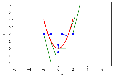
Almost 10 years ago I wrote about finding the minimum distance from a point to a curve using a constrained optimization. At that time, the way to do this used scipy.optimize.fmin_coblya. I learned today from a student, that sometimes this method fails! I reproduce the code here, updated for Python 3, some style updates, and to show it does indeed fail sometimes, notably when the point is "outside" the parabola.

import numpy as np
import matplotlib.pyplot as plt
from scipy.optimize import fmin_cobyla

def f(x):
    return x**2

for P in np.array([[0.5, 2],
                   [2, 2],
                   [-1, 2],
                   [-2, 2],
                   [0, 0.5],
                   [0, -0.5]]):
    
    def objective(X):
        X = np.array(X)
        return np.linalg.norm(X - P)

    def c1(X):
        x,y = X
        return f(x) - y

    X = fmin_cobyla(objective, x0=[P[0], f(P[0])], cons=[c1])

    print(f'The minimum distance is {objective(X):1.2f}. Constraint satisfied = {c1(X) < 1e-6}')

    # Verify the vector to this point is normal to the tangent of the curve
    # position vector from curve to point
    v1 = np.array(P) - np.array(X)
    # position vector
    v2 = np.array([1, 2.0 * X[0]])
    print('dot(v1, v2) = ', np.dot(v1, v2))

    x = np.linspace(-2, 2, 100)

    plt.plot(x, f(x), 'r-', label='f(x)')
    plt.plot(P[0], P[1], 'bo', label='point')
    plt.plot([P[0], X[0]], [P[1], X[1]], 'b-', label='shortest distance')
    plt.plot([X[0], X[0] + 1], [X[1], X[1] + 2.0 * X[0]], 'g-', label='tangent')
    plt.axis('equal')
    plt.xlabel('x')
    plt.ylabel('y')    

The minimum distance is 0.86. Constraint satisfied = True dot(v1, v2) = 0.0002913487659186309 The minimum distance is 0.00. Constraint satisfied = False dot(v1, v2) = 0.00021460906432962284 The minimum distance is 0.39. Constraint satisfied = True dot(v1, v2) = 0.00014271520451364372 The minimum distance is 0.00. Constraint satisfied = False dot(v1, v2) = -0.0004089466778209598 The minimum distance is 0.50. Constraint satisfied = True dot(v1, v2) = 1.9999998429305957e-12 The minimum distance is 0.00. Constraint satisfied = False dot(v1, v2) = 8.588744170160093e-06

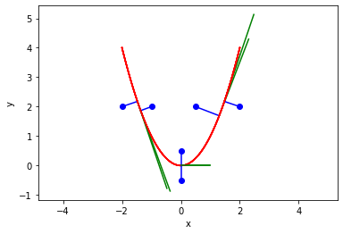
So, sure enough, the optimizer is failing to find a solution that meets the constraint. It is strange it does not work on the outside. That is almost certainly an algorithm problem. Here we solve it nearly identically with the more modern scipy.optimize.minimize function, and it converges every time.

from scipy.optimize import minimize

for P in np.array([[0.5, 2],
                   [2, 2],
                   [-1, 2],
                   [-2, 2],
                   [0, 0.5],
                   [0, -0.5]]):
    
    def objective(X):
        X = np.array(X)
        return np.linalg.norm(X - P)

    def c1(X):
        x,y = X
        return f(x) - y

    sol = minimize(objective, x0=[P[0], f(P[0])], constraints={'type': 'eq', 'fun': c1})
    X = sol.x

    print(f'The minimum distance is {objective(X):1.2f}. Constraint satisfied = {sol.status < 1e-6}')

    # Verify the vector to this point is normal to the tangent of the curve
    # position vector from curve to point
    v1 = np.array(P) - np.array(X)
    # position vector
    v2 = np.array([1, 2.0 * X[0]])
    print('dot(v1, v2) = ', np.dot(v1, v2))

    x = np.linspace(-2, 2, 100)

    plt.plot(x, f(x), 'r-', label='f(x)')
    plt.plot(P[0], P[1], 'bo', label='point')
    plt.plot([P[0], X[0]], [P[1], X[1]], 'b-', label='shortest distance')
    plt.plot([X[0], X[0] + 1], [X[1], X[1] + 2.0 * X[0]], 'g-', label='tangent')
    plt.axis('equal')
    plt.xlabel('x')
    plt.ylabel('y')

The minimum distance is 0.86. Constraint satisfied = True dot(v1, v2) = 1.0701251773603815e-08 The minimum distance is 0.55. Constraint satisfied = True dot(v1, v2) = -0.0005793028003104883 The minimum distance is 0.39. Constraint satisfied = True dot(v1, v2) = -1.869272921939391e-05 The minimum distance is 0.55. Constraint satisfied = True dot(v1, v2) = 0.0005792953298950909 The minimum distance is 0.50. Constraint satisfied = True dot(v1, v2) = 0.0 The minimum distance is 0.50. Constraint satisfied = True dot(v1, v2) = 0.0

There is no wisdom in fixing the first problem, here I just tried a newer optimization method. Out of the box with default settings it just worked. I did learn the answer is sensitive to the initial guess, so it could make sense to sample the function and find the point that is closest as the initial guess, but here the simple heuristic guess I used worked fine.

Copyright (C) 2023 by John Kitchin. See the License for information about copying.

org-mode source

Org-mode version = 9.5.5

Discuss on Twitter
« Previous Page -- Next Page »