Vibrational frequencies:PROPERTIES:

Vibrational frequencies:PROPERTIES:#

index:vibrations

Manual calculation of vibrational frequency#

The principle idea in calculating vibrational frequencies is that we consider a molecular system as masses connected by springs. If the springs are Hookean, e.g. the force is proportional to the displacement, then we can readily solve the equations of motion and find that the vibrational frequencies are related to the force constants and the masses of the atoms. For example, in a simple molecule like CO where there is only one spring, the frequency is:

\(\nu = \frac{1}{2\pi}\sqrt{k/\mu}\) where \(\frac{1}{\mu} = \frac{1}{m_C} + \frac{1}{m_O}\) and \(k\) is the spring constant. We will compute the value of \(k\) from DFT calculations as follows:

\(k = \frac{\partial^2E}{\partial x^2}\) at the equilibrium bond length. We actually already have the data to do this from [BROKEN LINK: *Manual%20determination%20of%20a%20bond%20length]. We only need to fit an equation to the energy vs. bond-length data, find the minimum energy bond-length, and then evaluate the second derivative of the fitted function at the minimum. We will use a cubic polynomial for demonstration here. Polynomials are numerically convenient because they are easy to fit, and it is trivial to get the roots and derivatives of the polynomials, as well as to evaluate them at other points using func:numpy.polyfit, func:numpy.polyder, and func:numpy.polyval.

from ase.io import read
import numpy as np
from ase import units
import os

bond_lengths = [1.05, 1.1, 1.15, 1.2, 1.25]
energies = []

for d in bond_lengths:
    outcar = 'molecules/co-{0}/OUTCAR'.format(d)
    if os.path.exists(outcar):
        atoms = read(outcar)
        energies.append(atoms.get_potential_energy())
    else:
        energies.append(np.nan)

# compute frequency from second derivative
pars = np.polyfit(bond_lengths, energies, 3)
# E = a*x^3 + b*x^2 + c*x + d
# dE/dx = 3*a*x^2 + 2*b*x + c
# d2E/dx2 = 6*a*x + 2*b
a, b, c, d = pars

# find minimum: dE/dx = 0
roots = np.roots([3*a, 2*b, c])
x_min = roots[(roots > 1.0) & (roots < 1.3)][0].real

# second derivative at minimum (force constant)
d2Edx2 = 6*a*x_min + 2*b  # eV/Angstrom^2

# convert to frequency
# omega = sqrt(k/mu)
mu = (12.0 * 16.0)/(12.0 + 16.0) * units._amu  # reduced mass in kg
k = d2Edx2 * units._e / (1e-10)**2  # convert to J/m^2

omega = np.sqrt(k/mu)  # rad/s
freq_Hz = omega / (2*np.pi)
freq_cm = freq_Hz / (100 * 299792458)  # cm^-1

print(f'Equilibrium bond length: {x_min:.4f} Angstrom')
print(f'Force constant: {d2Edx2:.2f} eV/Angstrom^2')
print(f'Vibrational frequency: {freq_cm:.0f} cm^-1')
print('(Experimental CO stretch: ~2143 cm^-1)')

Equilibrium bond length: 1.1444 Angstrom
Force constant: 116.14 eV/Angstrom^2
Vibrational frequency: 2146 cm^-1
(Experimental CO stretch: ~2143 cm^-1)

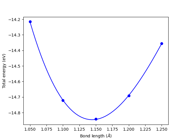
This result is in good agreement with experiment. The procedure described above is basically how many vibrational calculations are performed. With more atoms, you have to determine a force constant matrix and diagonalize it. For more details, see cite:wilson1955. In practice, we usually allow a packaged code to automate this, which we cover later.

We now consider how much energy is in this vibration. This is commonly called zero-point energy (ZPE) and it is defined as \(E_{ZPE} = \frac{1}{2} h \nu\) for a single mode, and \(h\) is Planck’s constant (4.135667516e-15 eV/s).

c = 3e10  # speed of light cm/s
h = 4.135667516e-15  # eV*s

nu = 2143.6076625*c  # 1/s

E_zpe = 0.5*h*nu

print('E_ZPE = {0:1.3f} eV'.format(E_zpe))

E_ZPE = 0.133 eV

This is a reasonable amount of energy! Zero-point energy increases with increasing vibrational frequency, and tends to be very important for small atoms.

A final note is that this analysis is in the “harmonic approximation”. The frequency equation is the solution to a harmonic oscillator. If the spring is non-linear, then there are anharmonic effects that may become important, especially at higher temperatures.

Automated vibrational calculations#

VASP has built-in capability for performing vibrational calculations. We access the capability by using a new value for incar:IBRION. The values of 5 and 6 calculated the Hessian matrix using finite differences. For IBRION=5, all atoms that are not constrained are displaced. For IBRION=6, only symmetry inequivalent displacements are considered, which makes the calculations slightly cheaper. You can specify the number of displacements with incar:NFREE. The default number of displacements is 2. You can also specify the size of the displacement with incar:POTIM (the default is 0.015 Å).

from ase.io import read
import os
# <<water-vib>>
# adapted from http://cms.mpi.univie.ac.at/wiki/index.php/H2O_vibration
from ase import Atoms, Atom
from vasp import Vasp
import ase.units

atoms = Atoms([Atom('H', [0.5960812,  -0.7677068,   0.0000000]),
               Atom('O', [0.0000000,   0.0000000,   0.0000000]),
               Atom('H', [0.5960812,   0.7677068,   0.0000000])],
              cell=(8, 8, 8))
atoms.center()

calc = Vasp(label='molecules/h2o_vib',
            xc='PBE',
            encut=350,
            ibrion=5,
            nfree=2,
            potim=0.015,
            ediff=1e-8,
            nsw=1,
            atoms=atoms)

energies, modes = calc.get_vibrational_modes()
print('energies\n========')
for i, e in enumerate(energies):
    print(f'{i:02d}: {e} 1/cm')
    

energies
========
3800.73575 1/cm
3686.514737 1/cm
1580.750273 1/cm
38.427236 1/cm
18.744884 1/cm
-2.488176 1/cm
-107.571746 1/cm
-114.207867 1/cm
-144.068332 1/cm

Note we get 9 frequencies here. Water has 3 atoms, with three degrees of freedom each, leading to 9 possible combinations of collective motions. Three of those collective motions are translations, i.e. where all atoms move in the same direction (either \(x\), \(y\) or \(z\)) and there is no change in the total energy of the molecule. Another three of those motions are rotations, which also do not change the total energy of the molecule. That leaves 3N-6 = 3 degrees of vibrational freedom where some or all of the bonds are stretched, resulting in a change in the total energy. The modes of water vibration are (with our calculated values in parentheses):

a symmetric stretch at 3657 cm^-1 (3723)
an asymmetric stretch at 3756 cm^-1 (3836)
and a bending mode at 1595 cm^-1 (1583)

http://webbook.nist.gov/cgi/cbook.cgi?ID=C7732185&Mask=800#Electronic-Spec

The results are not too far off, and more accurate frequencies may be possible using tighter tolerance on [BROKEN LINK: incar:POTIM], or by using [BROKEN LINK: incar:IBRION]=7 or 8.

Let us briefly discuss how to determine which vectors are vibrations and which are rotations or translations. One way is to visualize the modes. The vibrations are easy to spot. The rotations/translations are not always cleanly separable. This is an issue of accuracy and convergence. We usually do not worry about this because these modes are usually not important.

mode 0 is an asymmetric stretch
mode 1 is a symmetric stretch
mode 2 is a bending mode
mode 3 is a mixed translation/rotation
mode 4 is a rotation
mode 5 is a translation
mode 6 is a rotation
mode 7 is a partial translation
mode 8 is a rotation

# <<h2o-vib-vis>>
from vasp import Vasp
from ase.io import read
import numpy as np
import os

# Read atoms from existing calculation
contcar = 'molecules/h2o_vib/CONTCAR'
if os.path.exists(contcar):
    atoms = read(contcar, format='vasp')
    calc = Vasp(label='molecules/h2o_vib', atoms=atoms)
    energies, modes = calc.get_vibrational_modes()
    print('Vibrational frequencies (cm^-1):')
    for j, e in enumerate(energies):
        if e > 100:  # Only show real vibrational modes
            print(f'  Mode {j+1}: {e:.1f} cm^-1')
else:
    print('H2O vibration calculation not found')

Vibrational frequencies (cm^-1):
  Mode 1: 3800.7 cm^-1
  Mode 2: 3686.5 cm^-1
  Mode 3: 1580.8 cm^-1

See http://www.gaussian.com/g_whitepap/vib.htmfor a more quantitative discussion of these modes, identifying them, and a method to project the rotations and translations out of the Hessian matrix.

Zero-point energy for multiple modes#

For a molecule with lots of vibrational modes the zero-point energy is defined as the sum over all the vibrational modes:

\(E_{ZPE} = \sum_i \frac{1}{2} h \nu_i\)

Here is an example for water. Note we do not sum over the imaginary modes. We should also ignore the rotational and translational modes (some of those are imaginary, but some are just small).

from vasp import Vasp
from ase.io import read
import numpy as np
import os

c = 3e10  # speed of light cm/s
h = 4.135667516e-15  # eV/s

# first, get the frequencies
contcar = 'molecules/h2o_vib/CONTCAR'
if os.path.exists(contcar):
    atoms = read(contcar, format='vasp')
    calc = Vasp(label='molecules/h2o_vib', atoms=atoms)
    freq = calc.get_vibrational_frequencies()
    
    ZPE = 0.0
    for f in freq:
        if not np.isnan(f) and f > 0:  # only real frequencies
            nu = f * c  # convert cm^-1 to Hz (f * c)
            ZPE += 0.5 * h * nu
    
    print(f'Vibrational frequencies (cm^-1): {freq}')
    print(f'Zero-point energy: {ZPE:.4f} eV')
else:
    print('H2O vibration calculation not found')

Vibrational frequencies (cm^-1): [ 3.80073575e+03  3.68651474e+03  1.58075027e+03  3.84272360e+01
  1.87448840e+01 -2.48817600e+00 -1.07571746e+02 -1.14207867e+02
 -1.44068332e+02]
Zero-point energy: 0.5661 eV

Note the zero-point energy of water is also fairly high (more than 0.5 eV). That is because of the high frequency O-H stretches.

Vibrational frequencies:PROPERTIES:

Contents

Vibrational frequencies:PROPERTIES:#

Manual calculation of vibrational frequency#

Automated vibrational calculations#

Zero-point energy for multiple modes#