The Gibbs free energy of a reacting mixture and the equilibrium composition

| categories: optimization | tags: thermodynamics, reaction engineering

Table of Contents

Matlab post

In this post we derive the equations needed to find the equilibrium composition of a reacting mixture. We use the method of direct minimization of the Gibbs free energy of the reacting mixture.

The Gibbs free energy of a mixture is defined as \(G = \sum\limits_j \mu_j n_j\) where \(\mu_j\) is the chemical potential of species \(j\), and it is temperature and pressure dependent, and \(n_j\) is the number of moles of species \(j\).

We define the chemical potential as \(\mu_j = G_j^\circ + RT\ln a_j\), where \(G_j^\circ\) is the Gibbs energy in a standard state, and \(a_j\) is the activity of species \(j\) if the pressure and temperature are not at standard state conditions.

If a reaction is occurring, then the number of moles of each species are related to each other through the reaction extent \(\epsilon\) and stoichiometric coefficients: \(n_j = n_{j0} + \nu_j \epsilon\). Note that the reaction extent has units of moles.

Combining these three equations and expanding the terms leads to:

$$G = \sum\limits_j n_{j0}G_j^\circ +\sum\limits_j \nu_j G_j^\circ \epsilon +RT\sum\limits_j(n_{j0} + \nu_j\epsilon)\ln a_j $$

The first term is simply the initial Gibbs free energy that is present before any reaction begins, and it is a constant. It is difficult to evaluate, so we will move it to the left side of the equation in the next step, because it does not matter what its value is since it is a constant. The second term is related to the Gibbs free energy of reaction: \(\Delta_rG = \sum\limits_j \nu_j G_j^\circ\). With these observations we rewrite the equation as:

$$G - \sum\limits_j n_{j0}G_j^\circ = \Delta_rG \epsilon +RT\sum\limits_j(n_{j0} + \nu_j\epsilon)\ln a_j $$

Now, we have an equation that allows us to compute the change in Gibbs free energy as a function of the reaction extent, initial number of moles of each species, and the activities of each species. This difference in Gibbs free energy has no natural scale, and depends on the size of the system, i.e. on \(n_{j0}\). It is desirable to avoid this, so we now rescale the equation by the total initial moles present, \(n_{T0}\) and define a new variable \(\epsilon' = \epsilon/n_{T0}\), which is dimensionless. This leads to:

$$ \frac{G - \sum\limits_j n_{j0}G_j^\circ}{n_{T0}} = \Delta_rG \epsilon' + RT \sum\limits_j(y_{j0} + \nu_j\epsilon')\ln a_j $$

where \(y_{j0}\) is the initial mole fraction of species \(j\) present. The mole fractions are intensive properties that do not depend on the system size. Finally, we need to address \(a_j\). For an ideal gas, we know that \(A_j = \frac{y_j P}{P^\circ}\), where the numerator is the partial pressure of species \(j\) computed from the mole fraction of species \(j\) times the total pressure. To get the mole fraction we note:

$$y_j = \frac{n_j}{n_T} = \frac{n_{j0} + \nu_j \epsilon}{n_{T0} + \epsilon \sum\limits_j \nu_j} = \frac{y_{j0} + \nu_j \epsilon'}{1 + \epsilon'\sum\limits_j \nu_j} $$

This finally leads us to an equation that we can evaluate as a function of reaction extent:

$$ \frac{G - \sum\limits_j n_{j0}G_j^\circ}{n_{T0}} = \widetilde{\widetilde{G}} = \Delta_rG \epsilon' + RT\sum\limits_j(y_{j0} + \nu_j\epsilon') \ln\left(\frac{y_{j0}+\nu_j\epsilon'}{1+\epsilon'\sum\limits_j\nu_j} \frac{P}{P^\circ}\right) $$

we use a double tilde notation to distinguish this quantity from the quantity derived by Rawlings and Ekerdt which is further normalized by a factor of \(RT\). This additional scaling makes the quantities dimensionless, and makes the quantity have a magnitude of order unity, but otherwise has no effect on the shape of the graph.

Finally, if we know the initial mole fractions, the initial total pressure, the Gibbs energy of reaction, and the stoichiometric coefficients, we can plot the scaled reacting mixture energy as a function of reaction extent. At equilibrium, this energy will be a minimum. We consider the example in Rawlings and Ekerdt where isobutane (I) reacts with 1-butene (B) to form 2,2,3-trimethylpentane (P). The reaction occurs at a total pressure of 2.5 atm at 400K, with equal molar amounts of I and B. The standard Gibbs free energy of reaction at 400K is -3.72 kcal/mol. Compute the equilibrium composition.

import numpy as np

R = 8.314
P = 250000  # Pa
P0 = 100000 # Pa, approximately 1 atm
T = 400 # K

Grxn = -15564.0 #J/mol
yi0 = 0.5; yb0 = 0.5; yp0 = 0.0; # initial mole fractions

yj0 = np.array([yi0, yb0, yp0])
nu_j = np.array([-1.0, -1.0, 1.0])   # stoichiometric coefficients

def Gwigglewiggle(extentp):
    diffg = Grxn * extentp
    sum_nu_j = np.sum(nu_j)
    for i,y in enumerate(yj0):
        x1 = yj0[i] + nu_j[i] * extentp
        x2 = x1 / (1.0 + extentp*sum_nu_j)
        diffg += R * T * x1 * np.log(x2 * P / P0)
    return diffg

There are bounds on how large \(\epsilon'\) can be. Recall that \(n_j = n_{j0} + \nu_j \epsilon\), and that \(n_j \ge 0\). Thus, \(\epsilon_{max} = -n_{j0}/\nu_j\), and the maximum value that \(\epsilon'\) can have is therefore \(-y_{j0}/\nu_j\) where \(y_{j0}>0\). When there are multiple species, you need the smallest \(epsilon'_{max}\) to avoid getting negative mole numbers.

epsilonp_max = min(-yj0[yj0 > 0] / nu_j[yj0 > 0])
epsilonp = np.linspace(1e-6, epsilonp_max, 1000);

import matplotlib.pyplot as plt

plt.plot(epsilonp,Gwigglewiggle(epsilonp))
plt.xlabel('$\epsilon$')
plt.ylabel('Gwigglewiggle')
plt.savefig('images/gibbs-minim-1.png')
>>> >>> >>> __main__:7: RuntimeWarning: divide by zero encountered in log
__main__:7: RuntimeWarning: invalid value encountered in multiply
[<matplotlib.lines.Line2D object at 0x10b1c7710>]
<matplotlib.text.Text object at 0x10b1c3d10>
<matplotlib.text.Text object at 0x10b1c9b90>

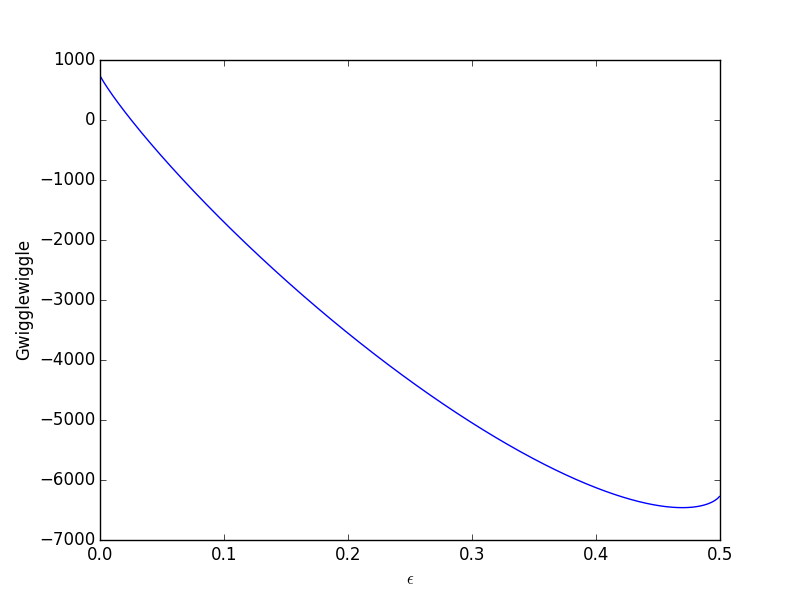
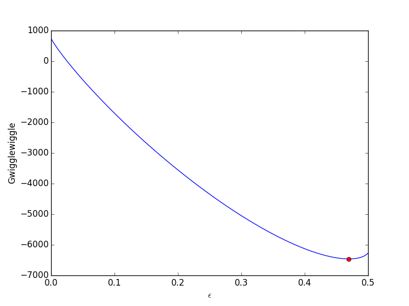
Now we simply minimize our Gwigglewiggle function. Based on the figure above, the miminum is near 0.45.

from scipy.optimize import fminbound

epsilonp_eq = fminbound(Gwigglewiggle, 0.4, 0.5)
print epsilonp_eq

plt.plot([epsilonp_eq], [Gwigglewiggle(epsilonp_eq)], 'ro')
plt.savefig('images/gibbs-minim-2.png')
>>> >>> 0.46959618249
>>> [<matplotlib.lines.Line2D object at 0x10d4d3e50>]

To compute equilibrium mole fractions we do this:

yi = (yi0 + nu_j[0]*epsilonp_eq) / (1.0 + epsilonp_eq*np.sum(nu_j))
yb = (yb0 + nu_j[1]*epsilonp_eq) / (1.0 + epsilonp_eq*np.sum(nu_j))
yp = (yp0 + nu_j[2]*epsilonp_eq) / (1.0 + epsilonp_eq*np.sum(nu_j))

print yi, yb, yp

# or this
y_j = (yj0 + np.dot(nu_j, epsilonp_eq)) / (1.0 + epsilonp_eq*np.sum(nu_j))
print y_j
>>> >>> >>> 0.0573220186324 0.0573220186324 0.885355962735
>>> ... >>> [ 0.05732202  0.05732202  0.88535596]

\(K = \frac{a_P}{a_I a_B} = \frac{y_p P/P^\circ}{y_i P/P^\circ y_b P/P^\circ} = \frac{y_P}{y_i y_b}\frac{P^\circ}{P}\).

We can express the equilibrium constant like this :\(K = \prod\limits_j a_j^{\nu_j}\), and compute it with a single line of code.

K = np.exp(-Grxn/R/T)
print 'K from delta G ',K
print 'K as ratio of mole fractions ',yp / (yi * yb) * P0 / P
print 'compact notation: ',np.prod((y_j * P / P0)**nu_j)
K from delta G  107.776294742
K as ratio of mole fractions  107.779200065
compact notation:  107.779200065

These results are very close, and only disagree because of the default tolerance used in identifying the minimum of our function. You could tighten the tolerances by setting options to the fminbnd function.

1 Summary

In this post we derived an equation for the Gibbs free energy of a reacting mixture and used it to find the equilibrium composition. In future posts we will examine some alternate forms of the equations that may be more useful in some circumstances.

Copyright (C) 2014 by John Kitchin. See the License for information about copying.

org-mode source

Org-mode version = 8.2.7c

Discuss on Twitter

The equal area method for the van der Waals equation

| categories: plotting | tags: thermodynamics

Table of Contents

Matlab post

When a gas is below its Tc the van der Waal equation oscillates. In the portion of the isotherm where \(\partial P_R/\partial V_r > 0\), the isotherm fails to describe real materials, which phase separate into a liquid and gas in this region.

Maxwell proposed to replace this region by a flat line, where the area above and below the curves are equal. Today, we examine how to identify where that line should be.

import numpy as np
import matplotlib.pyplot as plt

Tr = 0.9 # A Tr below Tc:  Tr = T/Tc
# analytical equation for Pr. This is the reduced form of the van der Waal
# equation.
def Prfh(Vr):
    return  8.0 / 3.0 * Tr / (Vr - 1.0 / 3.0) - 3.0 / (Vr**2)

Vr = np.linspace(0.5, 4, 100)  # vector of reduced volume
Pr = Prfh(Vr)                 # vector of reduced pressure

plt.plot(Vr,Pr)
plt.ylim([0, 2])
plt.xlabel('$V_R$')
plt.ylabel('$P_R$')
plt.savefig('images/maxwell-eq-area-1.png')
>>> >>> >>> >>> >>> >>> ... ... ... ... >>> >>> >>> >>> [<matplotlib.lines.Line2D object at 0x042FDAF0>]
(0, 2)
<matplotlib.text.Text object at 0x04237CB0>
<matplotlib.text.Text object at 0x042DC030>

The idea is to pick a Pr and draw a line through the EOS. We want the areas between the line and EOS to be equal on each side of the middle intersection. Let us draw a line on the figure at y = 0.65.

y = 0.65

plt.plot([0.5, 4.0], [y, y], 'k--')
plt.savefig('images/maxwell-eq-area-2.png')
>>> [<matplotlib.lines.Line2D object at 0x042FDCD0>]

To find the areas, we need to know where the intersection of the vdW eqn with the horizontal line. This is the same as asking what are the roots of the vdW equation at that Pr. We need all three intersections so we can integrate from the first root to the middle root, and then the middle root to the third root. We take advantage of the polynomial nature of the vdW equation, which allows us to use the roots command to get all the roots at once. The polynomial is \(V_R^3 - \frac{1}{3}(1+8 T_R/P_R) + 3/P_R - 1/P_R = 0\). We use the coefficients t0 get the roots like this.

vdWp = [1.0, -1. / 3.0 * (1.0 + 8.0 * Tr / y), 3.0 / y, - 1.0 / y]
v = np.roots(vdWp)
v.sort()
print v

plt.plot(v[0], y, 'bo', v[1], y, 'bo', v[2], y, 'bo')
plt.savefig('images/maxwell-eq-area-3.png')
>>> >>> [ 0.60286812  1.09743234  2.32534056]
>>> [<matplotlib.lines.Line2D object at 0x0439C570>, <matplotlib.lines.Line2D object at 0x043933B0>, <matplotlib.lines.Line2D object at 0x04393CB0>]

1 Compute areas

for A1, we need the area under the line minus the area under the vdW curve. That is the area between the curves. For A2, we want the area under the vdW curve minus the area under the line. The area under the line between root 2 and root 1 is just the width (root2 - root1)*y

from scipy.integrate import quad

A1, e1 = (v[1] - v[0]) * y - quad(Prfh,  v[0], v[1])
A2, e2 = quad(Prfh, v[1], v[2]) - (v[2] - v[1])* y 

print A1, A2
print e1, e2  # interesting these look so large
>>> >>> >>> >>> 0.063225945606 0.0580212098122
0.321466743765 -0.798140339268
from scipy.optimize import fsolve

def equal_area(y):
    Tr = 0.9
    vdWp = [1, -1.0 / 3 * ( 1.0 + 8.0 * Tr / y), 3.0 / y,  -1.0 / y]
    v = np.roots(vdWp)
    v.sort()
    A1 = (v[1] - v[0]) * y - quad(Prfh, v[0], v[1])
    A2 = quad(Prfh, v[1], v[2]) - (v[2] - v[1]) * y
    return  A1 - A2

y_eq, = fsolve(equal_area, 0.65)
print y_eq

Tr = 0.9
vdWp = [1, -1.0 / 3 * ( 1.0 + 8.0 * Tr / y_eq), 3.0 / y_eq,  -1.0 / y_eq]
v = np.roots(vdWp)
v.sort()

A1, e1 = (v[1] - v[0]) * y_eq - quad(Prfh,  v[0], v[1])
A2, e2 = quad(Prfh, v[1], v[2]) - (v[2] - v[1]) * y_eq

print A1, A2
>>> ... ... ... ... ... ... ... ... >>> >>> 0.646998351872
>>> >>> >>> >>> >>> >>> >>> >>> >>> 0.0617526473994 0.0617526473994

Now let us plot the equal areas and indicate them by shading.

fig = plt.gcf()
ax = fig.add_subplot(111)

ax.plot(Vr,Pr)

hline = np.ones(Vr.size) * y_eq

ax.plot(Vr, hline)
ax.fill_between(Vr, hline, Pr, where=(Vr >= v[0]) & (Vr <= v[1]), facecolor='gray')
ax.fill_between(Vr, hline, Pr, where=(Vr >= v[1]) & (Vr <= v[2]), facecolor='gray')

plt.text(v[0], 1, 'A1 = {0}'.format(A1))
plt.text(v[2], 1, 'A2 = {0}'.format(A2))
plt.xlabel('$V_R$')
plt.ylabel('$P_R$')
plt.title('$T_R$ = 0.9')

plt.savefig('images/maxwell-eq-area-4.png')
plt.savefig('images/maxwell-eq-area-4.svg')
>>> >>> [<matplotlib.lines.Line2D object at 0x043939D0>]
>>> >>> >>> [<matplotlib.lines.Line2D object at 0x043A7230>]
<matplotlib.collections.PolyCollection object at 0x047ADE70>
<matplotlib.collections.PolyCollection object at 0x047ADAB0>
>>> <matplotlib.text.Text object at 0x0438E730>
<matplotlib.text.Text object at 0x047B7930>
<matplotlib.text.Text object at 0x04237CB0>
<matplotlib.text.Text object at 0x042DC030>
<matplotlib.text.Text object at 0x042EBCD0>

Copyright (C) 2013 by John Kitchin. See the License for information about copying.

org-mode source

Discuss on Twitter

Constrained minimization to find equilibrium compositions

| categories: optimization | tags: thermodynamics, reaction engineering

adapated from Chemical Reactor analysis and design fundamentals, Rawlings and Ekerdt, appendix A.2.3.

Matlab post

The equilibrium composition of a reaction is the one that minimizes the total Gibbs free energy. The Gibbs free energy of a reacting ideal gas mixture depends on the mole fractions of each species, which are determined by the initial mole fractions of each species, the extent of reactions that convert each species, and the equilibrium constants.

Reaction 1: \(I + B \rightleftharpoons P1\)

Reaction 2: \(I + B \rightleftharpoons P2\)

Here we define the Gibbs free energy of the mixture as a function of the reaction extents.

import numpy as np

def gibbs(E):
    'function defining Gibbs free energy as a function of reaction extents'
    e1 = E[0]
    e2 = E[1]
    # known equilibrium constants and initial amounts
    K1 = 108; K2 = 284; P = 2.5
    yI0 = 0.5; yB0 = 0.5; yP10 = 0.0; yP20 = 0.0
    # compute mole fractions
    d = 1 - e1 - e2
    yI = (yI0 - e1 - e2) / d
    yB = (yB0 - e1 - e2) / d
    yP1 = (yP10 + e1) / d
    yP2 = (yP20 + e2) / d
    G = (-(e1 * np.log(K1) + e2 * np.log(K2)) +
         d * np.log(P) + yI * d * np.log(yI) +
         yB * d * np.log(yB) + yP1 * d * np.log(yP1) + yP2 * d * np.log(yP2))
    return G

The equilibrium constants for these reactions are known, and we seek to find the equilibrium reaction extents so we can determine equilibrium compositions. The equilibrium reaction extents are those that minimize the Gibbs free energy. We have the following constraints, written in standard less than or equal to form:

\(-\epsilon_1 \le 0\)

\(-\epsilon_2 \le 0\)

\(\epsilon_1 + \epsilon_2 \le 0.5\)

In Matlab we express this in matrix form as Ax=b where

\begin{equation} A = \left[ \begin{array}{cc} -1 & 0 \\ 0 & -1 \\ 1 & 1 \end{array} \right] \end{equation}

and

\begin{equation} b = \left[ \begin{array}{c} 0 \\ 0 \\ 0.5\end{array} \right] \end{equation}

Unlike in Matlab, in python we construct the inequality constraints as functions that are greater than or equal to zero when the constraint is met.

def constraint1(E):
    e1 = E[0]
    return e1


def constraint2(E):
    e2 = E[1]
    return e2


def constraint3(E):
    e1 = E[0]
    e2 = E[1]
    return 0.5 - (e1 + e2)

Now, we minimize.

from scipy.optimize import fmin_slsqp

X0 = [0.2, 0.2]
X = fmin_slsqp(gibbs, X0, ieqcons=[constraint1, constraint2, constraint3],
               bounds=((0.001, 0.499),
                       (0.001, 0.499)))
print(X)

print(gibbs(X))
Optimization terminated successfully.    (Exit mode 0)
            Current function value: -2.55942394906
            Iterations: 7
            Function evaluations: 31
            Gradient evaluations: 7
[ 0.13336503  0.35066486]
-2.55942394906

One way we can verify our solution is to plot the gibbs function and see where the minimum is, and whether there is more than one minimum. We start by making grids over the range of 0 to 0.5. Note we actually start slightly above zero because at zero there are some numerical imaginary elements of the gibbs function or it is numerically not defined since there are logs of zero there. We also set all elements where the sum of the two extents is greater than 0.5 to near zero, since those regions violate the constraints.

import numpy as np
import matplotlib.pyplot as plt

def gibbs(E):
    'function defining Gibbs free energy as a function of reaction extents'
    e1 = E[0]
    e2 = E[1]
    # known equilibrium constants and initial amounts
    K1 = 108; K2 = 284; P = 2.5;
    yI0 = 0.5; yB0 = 0.5; yP10 = 0.0; yP20 = 0.0;
    # compute mole fractions
    d = 1 - e1 - e2;
    yI = (yI0 - e1 - e2)/d;
    yB = (yB0 - e1 - e2)/d;
    yP1 = (yP10 + e1)/d;
    yP2 = (yP20 + e2)/d;
    G = (-(e1 * np.log(K1) + e2 * np.log(K2)) +
         d * np.log(P) + yI * d * np.log(yI) +
         yB * d * np.log(yB) + yP1 * d * np.log(yP1) + yP2 * d * np.log(yP2))
    return G


a = np.linspace(0.001, 0.5, 100)
E1, E2 = np.meshgrid(a,a)

sumE = E1 + E2
E1[sumE >= 0.5] = 0.00001
E2[sumE >= 0.5] = 0.00001

# now evaluate gibbs
G = np.zeros(E1.shape)
m,n = E1.shape

G = gibbs([E1, E2])

CS = plt.contour(E1, E2, G, levels=np.linspace(G.min(),G.max(),100))
plt.xlabel('$\epsilon_1$')
plt.ylabel('$\epsilon_2$')
plt.colorbar()

plt.plot([0.13336503],  [0.35066486], 'ro')

plt.savefig('images/gibbs-minimization-1.png')
plt.savefig('images/gibbs-minimization-1.svg')
plt.show()

You can see we found the minimum. We can compute the mole fractions pretty easily.

e1 = X[0];
e2 = X[1];

yI0 = 0.5; yB0 = 0.5; yP10 = 0; yP20 = 0; #initial mole fractions

d = 1 - e1 - e2;
yI = (yI0 - e1 - e2) / d
yB = (yB0 - e1 - e2) / d
yP1 = (yP10 + e1) / d
yP2 = (yP20 + e2) / d

print('y_I = {0:1.3f} y_B = {1:1.3f} y_P1 = {2:1.3f} y_P2 = {3:1.3f}'.format(yI,yB,yP1,yP2))
y_I = 0.031 y_B = 0.031 y_P1 = 0.258 y_P2 = 0.680

1 summary

I found setting up the constraints in this example to be more confusing than the Matlab syntax.

Copyright (C) 2016 by John Kitchin. See the License for information about copying.

org-mode source

Org-mode version = 8.2.10

Discuss on Twitter

Estimating the boiling point of water

| categories: uncategorized | tags: thermodynamics

Matlab post

I got distracted looking for Shomate parameters for ethane today, and came across this website on predicting the boiling point of water using the Shomate equations. The basic idea is to find the temperature where the Gibbs energy of water as a vapor is equal to the Gibbs energy of the liquid.

import matplotlib.pyplot as plt

Liquid water (\url{http://webbook.nist.gov/cgi/cbook.cgi?ID=C7732185&Units=SI&Mask=2#Thermo-Condensed})

# valid over 298-500

Hf_liq = -285.830   # kJ/mol
S_liq = 0.06995     # kJ/mol/K
shomateL = [-203.6060,
            1523.290,
           -3196.413,
            2474.455,
               3.855326,
            -256.5478,
            -488.7163,
            -285.8304]

Gas phase water (\url{http://webbook.nist.gov/cgi/cbook.cgi?ID=C7732185&Units=SI&Mask=1&Type=JANAFG&Table=on#JANAFG})

Interestingly, these parameters are listed as valid only above 500K. That means we have to extrapolate the values down to 298K. That is risky for polynomial models, as they can deviate substantially outside the region they were fitted to.

Hf_gas = -241.826  # kJ/mol
S_gas = 0.188835   # kJ/mol/K

shomateG = [30.09200,
             6.832514,
             6.793435,
            -2.534480,
             0.082139,
          -250.8810,
           223.3967,
          -241.8264]

Now, we wan to compute G for each phase as a function of T

import numpy as np

T = np.linspace(0, 200) + 273.15
t = T / 1000.0

sTT = np.vstack([np.log(t),
                 t,
                 (t**2) / 2.0,
                 (t**3) / 3.0,
                 -1.0 / (2*t**2),
                 0 * t,
                 t**0,
                 0 * t**0]).T / 1000.0

hTT = np.vstack([t,
                 (t**2)/2.0,
                 (t**3)/3.0,
                 (t**4)/4.0,
                 -1.0 / t,
                 1 * t**0,
                 0 * t**0,
                 -1 * t**0]).T

Gliq = Hf_liq + np.dot(hTT, shomateL) - T*(np.dot(sTT, shomateL))
Ggas = Hf_gas + np.dot(hTT, shomateG) - T*(np.dot(sTT, shomateG))
                 
from scipy.interpolate import interp1d
from scipy.optimize import fsolve

f = interp1d(T, Gliq - Ggas)
bp, = fsolve(f, 373)
print 'The boiling point is {0} K'.format(bp)
>>> >>> >>> >>> ... ... ... ... ... ... ... >>> >>> ... ... ... ... ... ... ... >>> >>> >>> >>> ... >>> >>> >>> >>> >>> The boiling point is 373.206081312 K
plt.figure(); plt.clf()
plt.plot(T-273.15, Gliq, T-273.15, Ggas)
plt.legend(['liquid water', 'steam'])

plt.xlabel('Temperature $^\circ$C')
plt.ylabel('$\Delta G$ (kJ/mol)')
plt.title('The boiling point is approximately {0:1.2f} $^\circ$C'.format(bp-273.15))
plt.savefig('images/boiling-water.png')
<matplotlib.figure.Figure object at 0x050D2E30>
[<matplotlib.lines.Line2D object at 0x051AB610>, <matplotlib.lines.Line2D object at 0x051B4C90>]
<matplotlib.legend.Legend object at 0x051B9030>
>>> <matplotlib.text.Text object at 0x0519E390>
<matplotlib.text.Text object at 0x050FB390>
<matplotlib.text.Text object at 0x050FBFB0>

1 Summary

The answer we get us 0.05 K too high, which is not bad considering we estimated it using parameters that were fitted to thermodynamic data and that had finite precision and extrapolated the steam properties below the region the parameters were stated to be valid for.

Copyright (C) 2013 by John Kitchin. See the License for information about copying.

org-mode source

Discuss on Twitter
« Previous Page