Meet the steam tables
Posted February 28, 2013 at 10:09 PM | categories: uncategorized | tags: steam, thermodynamics
Updated June 26, 2013 at 07:00 PM
Table of Contents
We will use the iapws module. Install it like this:
pip install iapws
Problem statement: A Rankine cycle operates using steam with the condenser at 100 degC, a pressure of 3.0 MPa and temperature of 600 degC in the boiler. Assuming the compressor and turbine operate reversibly, estimate the efficiency of the cycle.
Starting point in the Rankine cycle in condenser.
we have saturated liquid here, and we get the thermodynamic properties for the given temperature. In this python module, these properties are all in attributes of an IAPWS object created at a set of conditions.
1 Starting point in the Rankine cycle in condenser.
We have saturated liquid here, and we get the thermodynamic properties for the given temperature.
from iapws import IAPWS97

T1 = 100 + 273.15 #in K

sat_liquid1  = IAPWS97(T=T1, x=0) # x is the steam quality. 0 = liquid

P1 = sat_liquid1.P
s1 = sat_liquid1.s
h1 = sat_liquid1.h
v1 = sat_liquid1.v
2 Isentropic compression of liquid to point 2
The final pressure is given, and we need to compute the new temperatures, and enthalpy.
P2 = 3.0 # MPa
s2 = s1 # this is what isentropic means

sat_liquid2 = IAPWS97(P=P2, s=s1)
T2, = sat_liquid2.T
h2 = sat_liquid2.h

# work done to compress liquid. This is an approximation, since the
# volume does change a little with pressure, but the overall work here
# is pretty small so we neglect the volume change.
WdotP = v1*(P2 - P1);
print
print('The compressor work is: {0:1.4f} kJ/kg'.format(WdotP))
>>> >>> >>> >>> >>> >>> ... ... ... >>>
The compressor work is: 0.0030 kJ/kg
The compression work is almost negligible. This number is 1000 times smaller than we computed with Xsteam. I wonder what the units of v1 actually are.
3 Isobaric heating to T3 in boiler where we make steam
T3 = 600 + 273.15 # K
P3 = P2 # definition of isobaric
steam = IAPWS97(P=P3, T=T3)

h3 = steam.h
s3 = steam.s

Qb, = h3 - h2 # heat required to make the steam

print
print 'The boiler heat duty is: {0:1.2f} kJ/kg'.format(Qb)
>>> >>> >>> >>> >>> >>> >>> >>>
The boiler heat duty is: 3260.69 kJ/kg
4 Isentropic expansion through turbine to point 4
steam =  IAPWS97(P=P1, s=s3)
T4, = steam.T
h4 = steam.h
s4 = s3 # isentropic
Qc, = h4 - h1 # work required to cool from T4 to T1
print
print 'The condenser heat duty is {0:1.2f} kJ/kg'.format(Qc)
>>> >>> >>> >>>
The condenser heat duty is 2317.00 kJ/kg
5 To get from point 4 to point 1
WdotTurbine, = h4 - h3 # work extracted from the expansion
print('The turbine work is: {0:1.2f} kJ/kg'.format(WdotTurbine))
The turbine work is: -946.71 kJ/kg
6 Efficiency
This is a ratio of the work put in to make the steam, and the net work obtained from the turbine. The answer here agrees with the efficiency calculated in Sandler on page 135.
eta = -(WdotTurbine - WdotP) / Qb
print('The overall efficiency is {0:1.2%}.'.format(eta))
The overall efficiency is 29.03%.
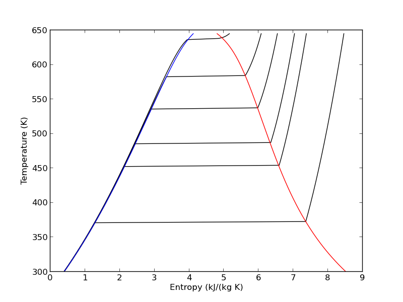
7 Entropy-temperature chart
The IAPWS module makes it pretty easy to generate figures of the steam tables. Here we generate an entropy-Temperature graph. We do this to illustrate the path of the Rankine cycle. We need to compute the values of steam entropy for a range of pressures and temperatures.
import numpy as np
import matplotlib.pyplot as plt

plt.figure()
plt.clf()
T = np.linspace(300, 372+273, 200) # range of temperatures
for P in [0.1, 1, 2, 5, 10, 20]: #MPa
    steam = [IAPWS97(T=t, P=P) for t in T]
    S = [s.s for s in steam]
    plt.plot(S, T, 'k-')

# saturated vapor and liquid entropy lines
svap = [s.s for s in [IAPWS97(T=t, x=1) for t in T]]
sliq = [s.s for s in [IAPWS97(T=t, x=0) for t in T]]

plt.plot(svap, T, 'r-')
plt.plot(sliq, T, 'b-')

plt.xlabel('Entropy (kJ/(kg K)')
plt.ylabel('Temperature (K)')
plt.savefig('images/iawps-steam.png')
>>> >>> <matplotlib.figure.Figure object at 0x000000000638BC18>
>>> >>> ... ... ... ... [<matplotlib.lines.Line2D object at 0x0000000007F9C208>]
[<matplotlib.lines.Line2D object at 0x0000000007F9C400>]
[<matplotlib.lines.Line2D object at 0x0000000007F9C8D0>]
[<matplotlib.lines.Line2D object at 0x0000000007F9CD30>]
[<matplotlib.lines.Line2D object at 0x0000000007F9E1D0>]
[<matplotlib.lines.Line2D object at 0x0000000007F9E630>]
... >>> >>> >>> [<matplotlib.lines.Line2D object at 0x0000000001FDCEB8>]
[<matplotlib.lines.Line2D object at 0x0000000007F9EA90>]
>>> <matplotlib.text.Text object at 0x0000000007F7BE48>
<matplotlib.text.Text object at 0x0000000007F855F8>
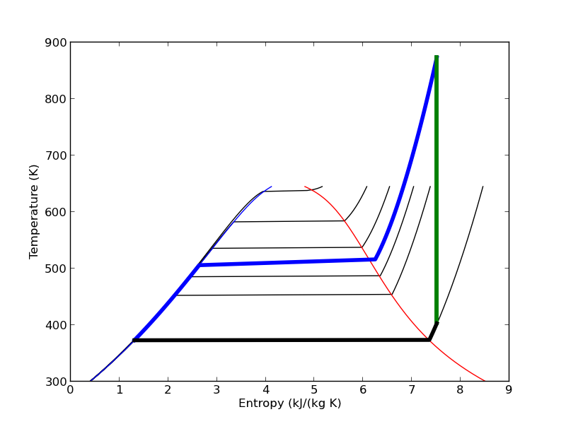
We can plot our Rankine cycle path like this. We compute the entropies along the non-isentropic paths.
T23 = np.linspace(T2, T3)
S23 = [s.s for s in [IAPWS97(P=P2, T=t) for t in T23]]

T41 = np.linspace(T4, T1 - 0.01) # subtract a tiny bit to make sure we get a liquid
S41 = [s.s for s in [IAPWS97(P=P1, T=t) for t in T41]]
And then we plot the paths.
plt.plot([s1, s2], [T1, T2], 'r-', lw=4) # Path 1 to 2
plt.plot(S23, T23, 'b-', lw=4) # path from 2 to 3 is isobaric
plt.plot([s3, s4], [T3, T4], 'g-', lw=4) # path from 3 to 4 is isentropic
plt.plot(S41, T41, 'k-', lw=4) # and from 4 to 1 is isobaric
plt.savefig('images/iawps-steam-2.png')
plt.savefig('images/iawps-steam-2.svg')
[<matplotlib.lines.Line2D object at 0x0000000008350908>]
[<matplotlib.lines.Line2D object at 0x00000000083358D0>]
[<matplotlib.lines.Line2D object at 0x000000000835BEB8>]
[<matplotlib.lines.Line2D object at 0x0000000008357160>]
8 Summary
This was an interesting exercise. On one hand, the tedium of interpolating the steam tables is gone. On the other hand, you still have to know exactly what to ask for to get an answer that is correct. The iapws interface is a little clunky, and takes some getting used to. It does not seem as robust as the Xsteam module I used in Matlab.
Copyright (C) 2013 by John Kitchin. See the License for information about copying.