Time dependent concentration in a first order reversible reaction in a batch reactor

| categories: ode | tags: reaction engineering

Matlab post

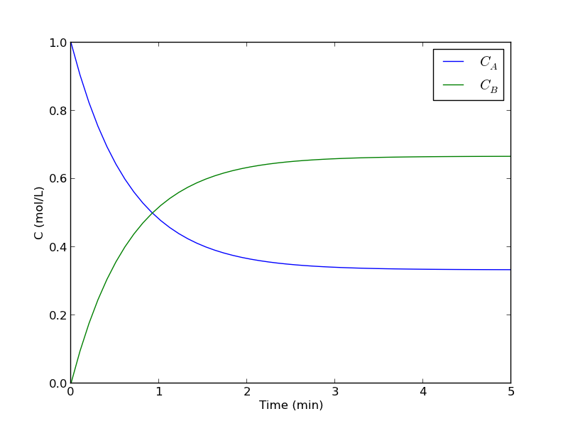
Given this reaction \(A \rightleftharpoons B\), with these rate laws:

forward rate law: \(-r_a = k_1 C_A\)

backward rate law: \(-r_b = k_{-1} C_B\)

plot the concentration of A vs. time. This example illustrates a set of coupled first order ODES.

from scipy.integrate import odeint
import numpy as np

def myode(C, t):
    # ra = -k1*Ca
    # rb = -k_1*Cb
    # net rate for production of A:  ra - rb
    # net rate for production of B: -ra + rb

    k1 = 1   # 1/min;
    k_1 = 0.5   # 1/min;

    Ca = C[0]
    Cb = C[1]

    ra = -k1 * Ca
    rb = -k_1 * Cb

    dCadt =  ra - rb
    dCbdt = -ra + rb

    dCdt = [dCadt, dCbdt]
    return dCdt

tspan = np.linspace(0, 5)

init = [1, 0]  # mol/L
C = odeint(myode, init, tspan)

Ca = C[:,0]
Cb = C[:,1]

import matplotlib.pyplot as plt
plt.plot(tspan, Ca, tspan, Cb)
plt.xlabel('Time (min)')
plt.ylabel('C (mol/L)')
plt.legend(['$C_A$', '$C_B$'])
plt.savefig('images/reversible-batch.png')

That is it. The main difference between this and Matlab is the order of arguments in odeint is different, and the ode function has differently ordered arguments.

Copyright (C) 2013 by John Kitchin. See the License for information about copying.

org-mode source

Discuss on Twitter

Solving integral equations with fsolve

| categories: nonlinear algebra | tags: reaction engineering

Original post in Matlab

Occasionally we have integral equations we need to solve in engineering problems, for example, the volume of plug flow reactor can be defined by this equation: \(V = \int_{Fa(V=0)}^{Fa} \frac{1}{r_a} dFa\) where \(r_a\) is the rate law. Suppose we know the reactor volume is 100 L, the inlet molar flow of A is 1 mol/L, the volumetric flow is 10 L/min, and \(r_a = -k Ca\), with \(k=0.23\) 1/min. What is the exit molar flow rate? We need to solve the following equation:

$$100 = \int_{Fa(V=0)}^{Fa} \frac{1}{-k Fa/\nu} dFa$$

We start by creating a function handle that describes the integrand. We can use this function in the quad command to evaluate the integral.

import numpy as np
from scipy.integrate import quad
from scipy.optimize import fsolve

k = 0.23
nu = 10.0
Fao = 1.0

def integrand(Fa):
    return -1.0 / (k * Fa / nu)

def func(Fa):
    integral,err = quad(integrand, Fao, Fa)
    return 100.0 - integral

vfunc = np.vectorize(func)

We will need an initial guess, so we make a plot of our function to get an idea.

import matplotlib.pyplot as plt

f = np.linspace(0.01, 1)
plt.plot(f, vfunc(f))
plt.xlabel('Molar flow rate')
plt.savefig('images/integral-eqn-guess.png')
plt.show()
>>> >>> [<matplotlib.lines.Line2D object at 0x964a910>]
<matplotlib.text.Text object at 0x961fe50>

Now we can see a zero is near Fa = 0.1, so we proceed to solve the equation.

Fa_guess = 0.1
Fa_exit, = fsolve(vfunc, Fa_guess)
print 'The exit concentration is {0:1.2f} mol/L'.format(Fa_exit / nu)
>>> The exit concentration is 0.01 mol/L

1 Summary notes

This example seemed a little easier in Matlab, where the quad function seemed to get automatically vectorized. Here we had to do it by hand.

Copyright (C) 2013 by John Kitchin. See the License for information about copying.

org-mode source

Discuss on Twitter

Integrating a batch reactor design equation

| categories: integration | tags: reaction engineering

For a constant volume batch reactor where \(A \rightarrow B\) at a rate of \(-r_A = k C_A^2\), we derive the following design equation for the length of time required to achieve a particular level of conversion :

\(t(X) = \frac{1}{k C_{A0}} \int_{X=0}^X \frac{dX}{(1-X)^2}\)

if \(k = 10^{-3}\) L/mol/s and \(C_{A0}\) = 1 mol/L, estimate the time to achieve 90% conversion.

We could analytically solve the integral and evaluate it, but instead we will numerically evaluate it using scipy.integrate.quad. This function returns two values: the evaluated integral, and an estimate of the absolute error in the answer.

from scipy.integrate import quad

def integrand(X):
    k = 1.0e-3
    Ca0 = 1.0  # mol/L
    return 1./(k*Ca0)*(1./(1-X)**2)

sol, abserr = quad(integrand, 0, 0.9)
print 't = {0} seconds ({1} hours)'.format(sol, sol/3600)
print 'Estimated absolute error = {0}'.format(abserr)
t = 9000.0 seconds (2.5 hours)
Estimated absolute error = 2.12203274482e-07

You can see the estimate error is very small compared to the solution.

Copyright (C) 2013 by John Kitchin. See the License for information about copying.

org-mode source

Discuss on Twitter

Integrating the batch reactor mole balance

| categories: ode | tags: reaction engineering

An alternative approach of evaluating an integral is to integrate a differential equation. For the batch reactor, the differential equation that describes conversion as a function of time is:

\(\frac{dX}{dt} = -r_A V/N_{A0}\).

Given a value of initial concentration, or volume and initial number of moles of A, we can integrate this ODE to find the conversion at some later time. We assume that \(X(t=0)=0\). We will integrate the ODE over a time span of 0 to 10,000 seconds.

from scipy.integrate import odeint
import numpy as np
import matplotlib.pyplot as plt

k = 1.0e-3
Ca0 = 1.0  # mol/L

def func(X, t):
    ra = -k * (Ca0 * (1 - X))**2
    return -ra / Ca0

X0 = 0
tspan = np.linspace(0,10000)

sol = odeint(func, X0, tspan)
plt.plot(tspan,sol)
plt.xlabel('Time (sec)')
plt.ylabel('Conversion')
plt.savefig('images/2013-01-06-batch-conversion.png')

You can read off of this figure to find the time required to achieve a particular conversion.

Copyright (C) 2013 by John Kitchin. See the License for information about copying.

org-mode source

Discuss on Twitter
« Previous Page