The Kitchin Research Group

Matlab post

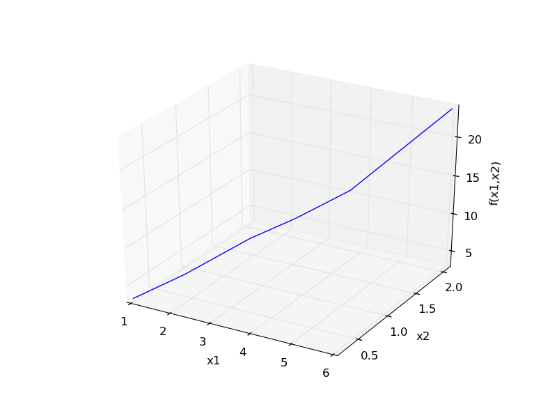
Fit the model f(x1,x2; a,b) = a*x1 + x2^b to the data given below. This model has two independent variables, and two parameters.

We want to do a nonlinear fit to find a and b that minimize the summed squared errors between the model predictions and the data. With only two variables, we can graph how the summed squared error varies with the parameters, which may help us get initial guesses. Let us assume the parameters lie in a range, here we choose 0 to 5. In other problems you would adjust this as needed.

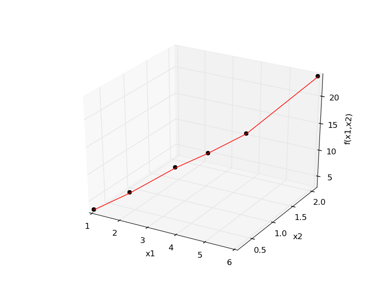
import numpy as np
from mpl_toolkits.mplot3d import Axes3D
import matplotlib.pyplot as plt

x1 = [1.0, 2.0, 3.0, 4.0, 5.0, 6.0]
x2 = [0.2, 0.4, 0.8, 0.9, 1.1, 2.1]
X = np.column_stack([x1, x2]) # independent variables

f = [ 3.3079,    6.6358,   10.3143,   13.6492,   17.2755,   23.6271]

fig = plt.figure()
ax = fig.gca(projection = '3d')

ax.plot(x1, x2, f)
ax.set_xlabel('x1')
ax.set_ylabel('x2')
ax.set_zlabel('f(x1,x2)')

plt.savefig('images/graphical-mulvar-1.png')


arange = np.linspace(0,5);
brange = np.linspace(0,5);

A,B = np.meshgrid(arange, brange)

def model(X, a, b):
    'Nested function for the model'
    x1 = X[:, 0]
    x2 = X[:, 1]
    
    f = a * x1 + x2**b
    return f

@np.vectorize
def errfunc(a, b):
    # function for the summed squared error
    fit = model(X, a, b)
    sse = np.sum((fit - f)**2)
    return sse

SSE = errfunc(A, B)

plt.clf()
plt.contourf(A, B, SSE, 50)
plt.plot([3.2], [2.1], 'ro')
plt.figtext( 3.4, 2.2, 'Minimum near here', color='r')

plt.savefig('images/graphical-mulvar-2.png')

guesses = [3.18, 2.02]

from scipy.optimize import curve_fit

popt, pcov = curve_fit(model, X, f, guesses)
print popt

plt.plot([popt[0]], [popt[1]], 'r*')
plt.savefig('images/graphical-mulvar-3.png')

print model(X, *popt)

fig = plt.figure()
ax = fig.gca(projection = '3d')

ax.plot(x1, x2, f, 'ko', label='data')
ax.plot(x1, x2, model(X, *popt), 'r-', label='fit')
ax.set_xlabel('x1')
ax.set_ylabel('x2')
ax.set_zlabel('f(x1,x2)')

plt.savefig('images/graphical-mulvar-4.png')

[ 3.21694798  1.9728254 ]
[  3.25873623   6.59792994  10.29473657  13.68011436  17.29161001
  23.62366445]

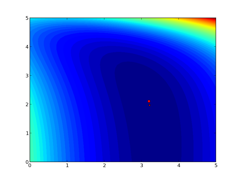
It can be difficult to figure out initial guesses for nonlinear fitting problems. For one and two dimensional systems, graphical techniques may be useful to visualize how the summed squared error between the model and data depends on the parameters.

Copyright (C) 2013 by John Kitchin. See the License for information about copying.

org-mode source

Matlab post

When a gas is below its Tc the van der Waal equation oscillates. In the portion of the isotherm where \(\partial P_R/\partial V_r > 0\), the isotherm fails to describe real materials, which phase separate into a liquid and gas in this region.

Maxwell proposed to replace this region by a flat line, where the area above and below the curves are equal. Today, we examine how to identify where that line should be.

import numpy as np
import matplotlib.pyplot as plt

Tr = 0.9 # A Tr below Tc:  Tr = T/Tc
# analytical equation for Pr. This is the reduced form of the van der Waal
# equation.
def Prfh(Vr):
    return  8.0 / 3.0 * Tr / (Vr - 1.0 / 3.0) - 3.0 / (Vr**2)

Vr = np.linspace(0.5, 4, 100)  # vector of reduced volume
Pr = Prfh(Vr)                 # vector of reduced pressure

plt.plot(Vr,Pr)
plt.ylim([0, 2])
plt.xlabel('$V_R$')
plt.ylabel('$P_R$')
plt.savefig('images/maxwell-eq-area-1.png')

>>> >>> >>> >>> >>> >>> ... ... ... ... >>> >>> >>> >>> [<matplotlib.lines.Line2D object at 0x042FDAF0>]
(0, 2)
<matplotlib.text.Text object at 0x04237CB0>
<matplotlib.text.Text object at 0x042DC030>

The idea is to pick a Pr and draw a line through the EOS. We want the areas between the line and EOS to be equal on each side of the middle intersection. Let us draw a line on the figure at y = 0.65.

y = 0.65

plt.plot([0.5, 4.0], [y, y], 'k--')
plt.savefig('images/maxwell-eq-area-2.png')

>>> [<matplotlib.lines.Line2D object at 0x042FDCD0>]

To find the areas, we need to know where the intersection of the vdW eqn with the horizontal line. This is the same as asking what are the roots of the vdW equation at that Pr. We need all three intersections so we can integrate from the first root to the middle root, and then the middle root to the third root. We take advantage of the polynomial nature of the vdW equation, which allows us to use the roots command to get all the roots at once. The polynomial is \(V_R^3 - \frac{1}{3}(1+8 T_R/P_R) + 3/P_R - 1/P_R = 0\). We use the coefficients t0 get the roots like this.

vdWp = [1.0, -1. / 3.0 * (1.0 + 8.0 * Tr / y), 3.0 / y, - 1.0 / y]
v = np.roots(vdWp)
v.sort()
print v

plt.plot(v[0], y, 'bo', v[1], y, 'bo', v[2], y, 'bo')
plt.savefig('images/maxwell-eq-area-3.png')

>>> >>> [ 0.60286812  1.09743234  2.32534056]
>>> [<matplotlib.lines.Line2D object at 0x0439C570>, <matplotlib.lines.Line2D object at 0x043933B0>, <matplotlib.lines.Line2D object at 0x04393CB0>]

from scipy.integrate import quad

A1, e1 = (v[1] - v[0]) * y - quad(Prfh,  v[0], v[1])
A2, e2 = quad(Prfh, v[1], v[2]) - (v[2] - v[1])* y 

print A1, A2
print e1, e2  # interesting these look so large

>>> >>> >>> >>> 0.063225945606 0.0580212098122
0.321466743765 -0.798140339268

from scipy.optimize import fsolve

def equal_area(y):
    Tr = 0.9
    vdWp = [1, -1.0 / 3 * ( 1.0 + 8.0 * Tr / y), 3.0 / y,  -1.0 / y]
    v = np.roots(vdWp)
    v.sort()
    A1 = (v[1] - v[0]) * y - quad(Prfh, v[0], v[1])
    A2 = quad(Prfh, v[1], v[2]) - (v[2] - v[1]) * y
    return  A1 - A2

y_eq, = fsolve(equal_area, 0.65)
print y_eq

Tr = 0.9
vdWp = [1, -1.0 / 3 * ( 1.0 + 8.0 * Tr / y_eq), 3.0 / y_eq,  -1.0 / y_eq]
v = np.roots(vdWp)
v.sort()

A1, e1 = (v[1] - v[0]) * y_eq - quad(Prfh,  v[0], v[1])
A2, e2 = quad(Prfh, v[1], v[2]) - (v[2] - v[1]) * y_eq

print A1, A2

>>> ... ... ... ... ... ... ... ... >>> >>> 0.646998351872
>>> >>> >>> >>> >>> >>> >>> >>> >>> 0.0617526473994 0.0617526473994

fig = plt.gcf()
ax = fig.add_subplot(111)

ax.plot(Vr,Pr)

hline = np.ones(Vr.size) * y_eq

ax.plot(Vr, hline)
ax.fill_between(Vr, hline, Pr, where=(Vr >= v[0]) & (Vr <= v[1]), facecolor='gray')
ax.fill_between(Vr, hline, Pr, where=(Vr >= v[1]) & (Vr <= v[2]), facecolor='gray')

plt.text(v[0], 1, 'A1 = {0}'.format(A1))
plt.text(v[2], 1, 'A2 = {0}'.format(A2))
plt.xlabel('$V_R$')
plt.ylabel('$P_R$')
plt.title('$T_R$ = 0.9')

plt.savefig('images/maxwell-eq-area-4.png')
plt.savefig('images/maxwell-eq-area-4.svg')

>>> >>> [<matplotlib.lines.Line2D object at 0x043939D0>]
>>> >>> >>> [<matplotlib.lines.Line2D object at 0x043A7230>]
<matplotlib.collections.PolyCollection object at 0x047ADE70>
<matplotlib.collections.PolyCollection object at 0x047ADAB0>
>>> <matplotlib.text.Text object at 0x0438E730>
<matplotlib.text.Text object at 0x047B7930>
<matplotlib.text.Text object at 0x04237CB0>
<matplotlib.text.Text object at 0x042DC030>
<matplotlib.text.Text object at 0x042EBCD0>

Copyright (C) 2013 by John Kitchin. See the License for information about copying.

org-mode source