Matlab post
It is an unknown fact that Picasso had a brief blue plotting period with Matlab before moving on to his more famous paintings. It started from irritation with the default colors available in Matlab for plotting. After watching his friend van Gogh cut off his own ear out of frustration with the ugly default colors, Picasso had to do something different.
import numpy as np
import matplotlib.pyplot as plt
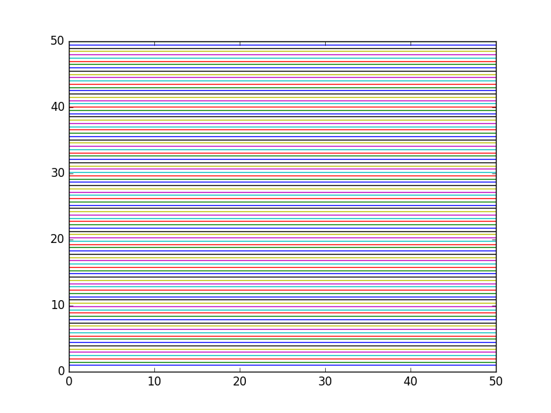
#this plots horizontal lines for each y value of m.
for m in np.linspace(1, 50, 100):
plt.plot([0, 50], [m, m])
plt.savefig('images/blues-1.png')
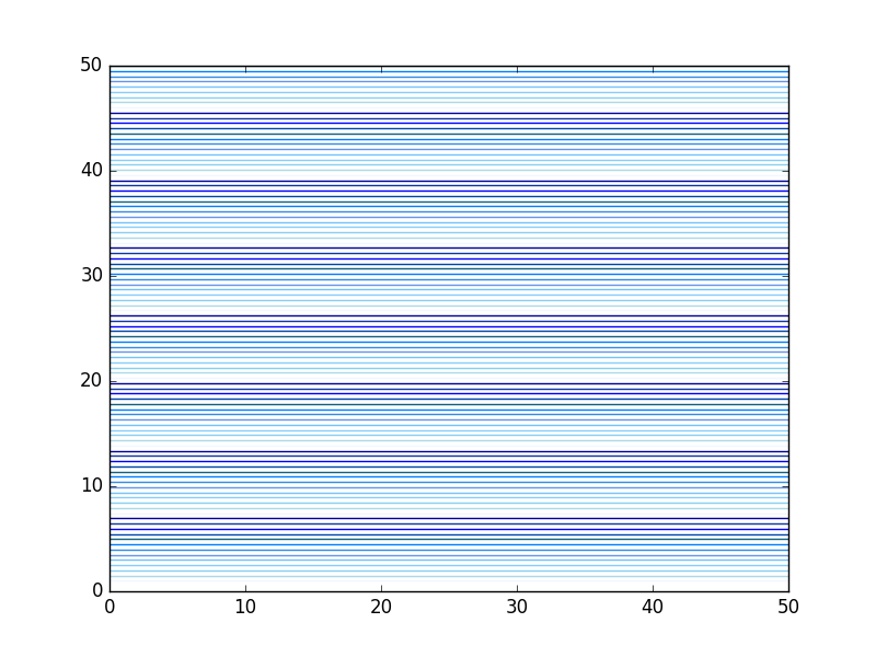
Picasso copied the table available at http://en.wikipedia.org/wiki/List_of_colors and parsed it into a dictionary of hex codes for new colors. That allowed him to specify a list of beautiful blues for his graph. Picasso eventually gave up on python as an artform, and moved on to painting.
import numpy as np
import matplotlib.pyplot as plt

c = {}
with open('color.table') as f:
    for line in f:
        fields = line.split('\t')
        colorname = fields[0].lower()
        hexcode = fields[1]
        c[colorname] = hexcode

names = c.keys()
names = sorted(names)

print(names)

blues = [c['alice blue'],
         c['light blue'],
         c['baby blue'],
         c['light sky blue'],
         c['maya blue'],
         c['cornflower blue'],
         c['bleu de france'],
         c['azure'],
         c['blue sapphire'],
         c['cobalt'],
         c['blue'],
         c['egyptian blue'],
         c['duke blue']]

ax = plt.gca()
ax.set_color_cycle(blues)

#this plots horizontal lines for each y value of m.
for i, m in enumerate(np.linspace(1, 50, 100)):
    plt.plot([0, 50], [m, m])

plt.savefig('images/blues-2.png')
['aero', 'aero blue', 'african violet', 'air force blue (raf)', 'air force blue (usaf)', 'air superiority blue', 'alabama crimson', 'alice blue', 'alizarin crimson', 'alloy orange', 'almond', 'amaranth', 'amazon', 'amber', 'american rose', 'amethyst', 'android green', 'anti-flash white', 'antique brass', 'antique bronze', 'antique fuchsia', 'antique ruby', 'antique white', 'ao (english)', 'apple green', 'apricot', 'aqua', 'aquamarine', 'army green', 'arsenic', 'arylide yellow', 'ash grey', 'asparagus', 'atomic tangerine', 'auburn', 'aureolin', 'aurometalsaurus', 'avocado', 'azure', 'azure mist/web', "b'dazzled blue", 'baby blue', 'baby blue eyes', 'baby pink', 'baby powder', 'baker-miller pink', 'ball blue', 'banana mania', 'banana yellow', 'barbie pink', 'barn red', 'battleship grey', 'bazaar', 'beau blue', 'beaver', 'beige', 'big dip o’ruby', 'bisque', 'bistre', 'bistre brown', 'bitter lemon', 'bitter lime', 'bittersweet', 'bittersweet shimmer', 'black', 'black bean', 'black leather jacket', 'black olive', 'blanched almond', 'blast-off bronze', 'bleu de france', 'blizzard blue', 'blond', 'blue', 'blue (crayola)', 'blue (munsell)', 'blue (ncs)', 'blue (pigment)', 'blue (ryb)', 'blue bell', 'blue sapphire', 'blue yonder', 'blue-gray', 'blue-green', 'blue-violet', 'blueberry', 'bluebonnet', 'blush', 'bole', 'bondi blue', 'bone', 'boston university red', 'bottle green', 'boysenberry', 'brandeis blue', 'brass', 'brick red', 'bright cerulean', 'bright green', 'bright lavender', 'bright maroon', 'bright pink', 'bright turquoise', 'bright ube', 'brilliant lavender', 'brilliant rose', 'brink pink', 'british racing green', 'bronze', 'bronze yellow', 'brown (traditional)', 'brown (web)', 'brown-nose', 'brunswick green', 'bubble gum', 'bubbles', 'buff', 'bulgarian rose', 'burgundy', 'burlywood', 'burnt orange', 'burnt sienna', 'burnt umber', 'byzantine', 'byzantium', 'cadet', 'cadet blue', 'cadet grey', 'cadmium green', 'cadmium orange', 'cadmium red', 'cadmium yellow', 'café au lait', 'café noir', 'cal poly green', 'cambridge blue', 'camel', 'cameo pink', 'camouflage green', 'canary yellow', 'candy apple red', 'candy pink', 'capri', 'caput mortuum', 'cardinal', 'caribbean green', 'carmine', 'carmine (m&p)', 'carmine pink', 'carmine red', 'carnation pink', 'carnelian', 'carolina blue', 'carrot orange', 'castleton green', 'catalina blue', 'catawba', 'cedar chest', 'ceil', 'celadon', 'celadon blue', 'celadon green', 'celeste (colour)', 'celestial blue', 'cerise', 'cerise pink', 'cerulean', 'cerulean blue', 'cerulean frost', 'cg blue', 'cg red', 'chamoisee', 'champagne', 'charcoal', 'charleston green', 'charm pink', 'chartreuse (traditional)', 'chartreuse (web)', 'cherry', 'cherry blossom pink', 'chestnut', 'china pink', 'china rose', 'chinese red', 'chinese violet', 'chocolate (traditional)', 'chocolate (web)', 'chrome yellow', 'cinereous', 'cinnabar', 'cinnamon', 'citrine', 'citron', 'claret', 'classic rose', 'cobalt', 'cocoa brown', 'coconut', 'coffee', 'columbia blue', 'congo pink', 'cool black', 'cool grey', 'copper', 'copper (crayola)', 'copper penny', 'copper red', 'copper rose', 'coquelicot', 'coral', 'coral pink', 'coral red', 'cordovan', 'corn', 'cornell red', 'cornflower blue', 'cornsilk', 'cosmic latte', 'cotton candy', 'cream', 'crimson', 'crimson glory', 'cyan', 'cyan (process)', 'cyber grape', 'cyber yellow', 'daffodil', 'dandelion', 'dark blue', 'dark blue-gray', 'dark brown', 'dark byzantium', 'dark candy apple red', 'dark cerulean', 'dark chestnut', 'dark coral', 'dark cyan', 'dark electric blue', 'dark goldenrod', 'dark gray', 'dark green', 'dark imperial blue', 'dark jungle green', 'dark khaki', 'dark lava', 'dark lavender', 'dark liver', 'dark liver (horses)', 'dark magenta', 'dark midnight blue', 'dark moss green', 'dark olive green', 'dark orange', 'dark orchid', 'dark pastel blue', 'dark pastel green', 'dark pastel purple', 'dark pastel red', 'dark pink', 'dark powder blue', 'dark raspberry', 'dark red', 'dark salmon', 'dark scarlet', 'dark sea green', 'dark sienna', 'dark sky blue', 'dark slate blue', 'dark slate gray', 'dark spring green', 'dark tan', 'dark tangerine', 'dark taupe', 'dark terra cotta', 'dark turquoise', 'dark vanilla', 'dark violet', 'dark yellow', 'dartmouth green', "davy's grey", 'debian red', 'deep carmine', 'deep carmine pink', 'deep carrot orange', 'deep cerise', 'deep champagne', 'deep chestnut', 'deep coffee', 'deep fuchsia', 'deep jungle green', 'deep lemon', 'deep lilac', 'deep magenta', 'deep mauve', 'deep moss green', 'deep peach', 'deep pink', 'deep ruby', 'deep saffron', 'deep sky blue', 'deep space sparkle', 'deep taupe', 'deep tuscan red', 'deer', 'denim', 'desert', 'desert sand', 'diamond', 'dim gray', 'dirt', 'dodger blue', 'dogwood rose', 'dollar bill', 'donkey brown', 'drab', 'duke blue', 'dust storm', 'earth yellow', 'ebony', 'ecru', 'eggplant', 'eggshell', 'egyptian blue', 'electric blue', 'electric crimson', 'electric cyan', 'electric green', 'electric indigo', 'electric lavender', 'electric lime', 'electric purple', 'electric ultramarine', 'electric violet', 'electric yellow', 'emerald', 'english green', 'english lavender', 'english red', 'english violet', 'eton blue', 'eucalyptus', 'fallow', 'falu red', 'fandango', 'fandango pink', 'fashion fuchsia', 'fawn', 'feldgrau', 'feldspar', 'fern green', 'ferrari red', 'field drab', 'fire engine red', 'firebrick', 'flame', 'flamingo pink', 'flattery', 'flavescent', 'flax', 'flirt', 'floral white', 'fluorescent orange', 'fluorescent pink', 'fluorescent yellow', 'folly', 'forest green (traditional)', 'forest green (web)', 'french beige', 'french bistre', 'french blue', 'french lilac', 'french lime', 'french mauve', 'french raspberry', 'french rose', 'french sky blue', 'french wine', 'fresh air', 'fuchsia', 'fuchsia (crayola)', 'fuchsia pink', 'fuchsia rose', 'fulvous', 'fuzzy wuzzy', 'gainsboro', 'gamboge', 'ghost white', 'giants orange', 'ginger', 'glaucous', 'glitter', 'go green', 'gold (metallic)', 'gold (web) (golden)', 'gold fusion', 'golden brown', 'golden poppy', 'golden yellow', 'goldenrod', 'granny smith apple', 'grape', 'gray', 'gray (html/css gray)', 'gray (x11 gray)', 'gray-asparagus', 'gray-blue', 'green (color wheel) (x11 green)', 'green (crayola)', 'green (html/css color)', 'green (munsell)', 'green (ncs)', 'green (pigment)', 'green (ryb)', 'green-yellow', 'grullo', 'guppie green', 'halayà úbe', 'han blue', 'han purple', 'hansa yellow', 'harlequin', 'harvard crimson', 'harvest gold', 'heart gold', 'heliotrope', 'hollywood cerise', 'honeydew', 'honolulu blue', "hooker's green", 'hot magenta', 'hot pink', 'hunter green', 'iceberg', 'icterine', 'illuminating emerald', 'imperial', 'imperial blue', 'imperial purple', 'imperial red', 'inchworm', 'india green', 'indian red', 'indian yellow', 'indigo', 'indigo (dye)', 'indigo (web)', 'international klein blue', 'international orange (aerospace)', 'international orange (engineering)', 'international orange (golden gate bridge)', 'iris', 'irresistible', 'isabelline', 'islamic green', 'italian sky blue', 'ivory', 'jade', 'japanese indigo', 'japanese violet', 'jasmine', 'jasper', 'jazzberry jam', 'jelly bean', 'jet', 'jonquil', 'june bud', 'jungle green', 'kelly green', 'kenyan copper', 'keppel', 'khaki (html/css) (khaki)', 'khaki (x11) (light khaki)', 'kobe', 'kobi', 'ku crimson', 'la salle green', 'languid lavender', 'lapis lazuli', 'laser lemon', 'laurel green', 'lava', 'lavender (floral)', 'lavender (web)', 'lavender blue', 'lavender blush', 'lavender gray', 'lavender indigo', 'lavender magenta', 'lavender mist', 'lavender pink', 'lavender purple', 'lavender rose', 'lawn green', 'lemon', 'lemon chiffon', 'lemon curry', 'lemon glacier', 'lemon lime', 'lemon meringue', 'lemon yellow', 'licorice', 'light apricot', 'light blue', 'light brown', 'light carmine pink', 'light coral', 'light cornflower blue', 'light crimson', 'light cyan', 'light fuchsia pink', 'light goldenrod yellow', 'light gray', 'light green', 'light khaki', 'light medium orchid', 'light moss green', 'light orchid', 'light pastel purple', 'light pink', 'light red ochre', 'light salmon', 'light salmon pink', 'light sea green', 'light sky blue', 'light slate gray', 'light steel blue', 'light taupe', 'light thulian pink', 'light yellow', 'lilac', 'lime (color wheel)', 'lime (web) (x11 green)', 'lime green', 'limerick', 'lincoln green', 'linen', 'lion', 'little boy blue', 'liver', 'liver (dogs)', 'liver (organ)', 'liver chestnut', 'lumber', 'lust', 'magenta', 'magenta (crayola)', 'magenta (dye)', 'magenta (pantone)', 'magenta (process)', 'magic mint', 'magnolia', 'mahogany', 'maize', 'majorelle blue', 'malachite', 'manatee', 'mango tango', 'mantis', 'mardi gras', 'maroon (crayola)', 'maroon (html/css)', 'maroon (x11)', 'mauve', 'mauve taupe', 'mauvelous', 'maya blue', 'meat brown', 'medium aquamarine', 'medium blue', 'medium candy apple red', 'medium carmine', 'medium champagne', 'medium electric blue', 'medium jungle green', 'medium lavender magenta', 'medium orchid', 'medium persian blue', 'medium purple', 'medium red-violet', 'medium ruby', 'medium sea green', 'medium sky blue', 'medium slate blue', 'medium spring bud', 'medium spring green', 'medium taupe', 'medium turquoise', 'medium tuscan red', 'medium vermilion', 'medium violet-red', 'mellow apricot', 'mellow yellow', 'melon', 'metallic seaweed', 'metallic sunburst', 'mexican pink', 'midnight blue', 'midnight green (eagle green)', 'midori', 'mikado yellow', 'mint', 'mint cream', 'mint green', 'misty rose', 'moccasin', 'mode beige', 'moonstone blue', 'mordant red 19', 'moss green', 'mountain meadow', 'mountbatten pink', 'msu green', 'mughal green', 'mulberry', 'mustard', 'myrtle green', 'sae/ece amber (color)']
Copyright (C) 2018 by John Kitchin. See the License for information about copying.
org-mode source
Org-mode version = 9.1.6