The Kitchin Research Group

There is a heat transfer problem where one needs to find the n^th root of the following equation: \(x J_1(x) - Bi J_0(x)=0\) where \(J_0\) and \(J_1\) are the Bessel functions of zero and first order, and \(Bi\) is the Biot number. We examine an approach to finding these roots.

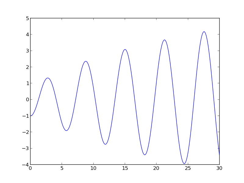
First, we plot the function.

from scipy.special import jn, jn_zeros
import matplotlib.pyplot as plt
import numpy as np

Bi = 1

def f(x):
    return x * jn(1, x) - Bi * jn(0, x)

X = np.linspace(0, 30, 200)
plt.plot(X, f(X))
plt.savefig('images/heat-transfer-roots-1.png')

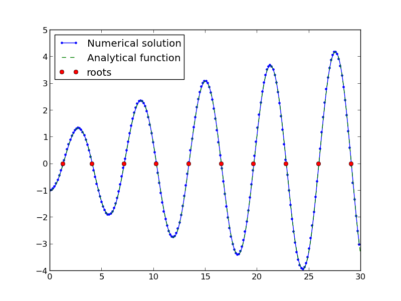
You can see there are many roots to this equation, and we want to be sure we get the n^{th} root. This function is pretty well behaved, so if you make a good guess about the solution you will get an answer, but if you make a bad guess, you may get the wrong root. We examine next a way to do it without guessing the solution. What we want is the solution to \(f(x) = 0\), but we want all the solutions in a given interval. We derive a new equation, \(f'(x) = 0\), with initial condition \(f(0) = f0\), and integrate the ODE with an event function that identifies all zeros of \(f\) for us. The derivative of our function is \(df/dx = d/dx(x J_1(x)) - Bi J'_0(x)\). It is known (http://www.markrobrien.com/besselfunct.pdf) that \(d/dx(x J_1(x)) = x J_0(x)\), and \(J'_0(x) = -J_1(x)\). All we have to do now is set up the problem and run it.

from pycse import *  # contains the ode integrator with events

from scipy.special import jn, jn_zeros
import matplotlib.pyplot as plt
import numpy as np

Bi = 1

def f(x):
    "function we want roots for"
    return x * jn(1, x) - Bi * jn(0, x)

def fprime(f, x):
    "df/dx"
    return x * jn(0, x) - Bi * (-jn(1, x))

def e1(f, x):
    "event function to find zeros of f"
    isterminal = False
    value = f
    direction = 0
    return value, isterminal, direction

f0 = f(0)
xspan = np.linspace(0, 30, 200)

x, fsol, XE, FE, IE = odelay(fprime, f0, xspan, events=[e1])

plt.plot(x, fsol, '.-', label='Numerical solution')
plt.plot(xspan, f(xspan), '--', label='Analytical function')
plt.plot(XE, FE, 'ro', label='roots')
plt.legend(loc='best')
plt.savefig('images/heat-transfer-roots-2.png')

for i, root in enumerate(XE):
    print 'root {0} is at {1}'.format(i, root)

plt.show()

root 0 is at 1.25578377377
root 1 is at 4.07947743741
root 2 is at 7.15579904465
root 3 is at 10.2709851256
root 4 is at 13.3983973869
root 5 is at 16.5311587137
root 6 is at 19.6667276775
root 7 is at 22.8039503455
root 8 is at 25.9422288192
root 9 is at 29.081221492

You can work this out once, and then you have all the roots in the interval and you can select the one you want.

Copyright (C) 2013 by John Kitchin. See the License for information about copying.

org-mode source