Nonlinear curve fitting by direct least squares minimization
Posted February 18, 2013 at 09:00 AM | categories: data analysis | tags:
Updated February 27, 2013 at 02:40 PM
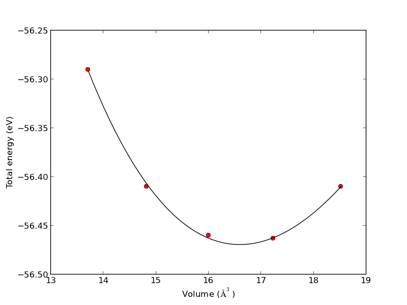
Here is an example of fitting a nonlinear function to data by direct minimization of the summed squared error.
from scipy.optimize import fmin
import numpy as np

volumes = np.array([13.71, 14.82, 16.0, 17.23, 18.52])

energies = np.array([-56.29, -56.41, -56.46, -56.463,-56.41])

def Murnaghan(parameters,vol):
    'From PRB 28,5480 (1983'
    E0 = parameters[0]
    B0 = parameters[1]
    BP = parameters[2]
    V0 = parameters[3]

    E = E0 + B0*vol/BP*(((V0/vol)**BP)/(BP-1)+1) - V0*B0/(BP-1.)

    return E

def objective(pars,vol):
    #we will minimize this function
    err =  energies - Murnaghan(pars,vol)
    return np.sum(err**2) #we return the summed squared error directly

x0 = [ -56., 0.54, 2., 16.5] #initial guess of parameters

plsq = fmin(objective,x0,args=(volumes,)) #note args is a tuple

print 'parameters = {0}'.format(plsq)

import matplotlib.pyplot as plt
plt.plot(volumes,energies,'ro')

#plot the fitted curve on top
x = np.linspace(min(volumes),max(volumes),50)
y = Murnaghan(plsq,x)
plt.plot(x,y,'k-')
plt.xlabel('Volume ($\AA^3$)')
plt.ylabel('Total energy (eV)')
plt.savefig('images/nonlinear-fitting-lsq.png')
Optimization terminated successfully.
         Current function value: 0.000020
         Iterations: 137
         Function evaluations: 240
parameters = [-56.46932645   0.59141447   1.9044796   16.59341303]
Copyright (C) 2013 by John Kitchin. See the License for information about copying.